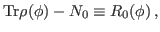
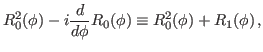
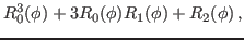
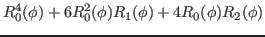
Kernels and Lipkin parameters up to sixth order
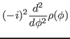
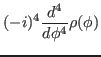
To calculate kernels  from derivatives of the overlap
kernel
from derivatives of the overlap
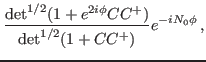
kernel  , in Eq. (5), we use the Onishi theorem [2]:
where  is the Thouless matrix.
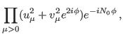
In the canonical basis of the Bogoliubov transformation, the above overlap is given as
is the Thouless matrix.
In the canonical basis of the Bogoliubov transformation, the above overlap is given as
where the label  is associated with one of the pair-conjugated canonical states
 . Then the
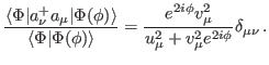
density matrix in canonical basis can be obtained as
. Then the
density matrix in canonical basis can be obtained as
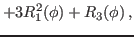
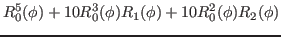
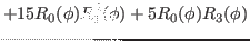
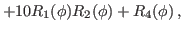
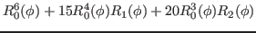
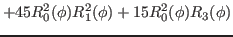
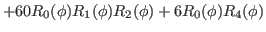
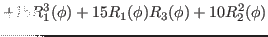
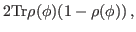
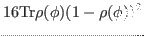
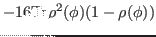
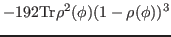
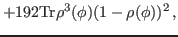
We then have the reduced kernels
 given as
 |
 |
 |
(20) |
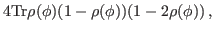
 |
|
 |
(21) |
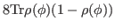
 |
|
 |
(22) |
 |
|
 |
|
| |
|
 |
(23) |
 |
 |
 |
|
| |
|
 |
|
| |
|
 |
(24) |
 |
|
 |
|
| |
|
 |
|
| |
|
 |
|
| |
|
 |
|
| |
|
 |
(25) |
where we used the definition
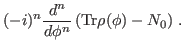
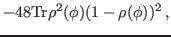
Derivatives of the density matrix  (19) can be calculated as,
which gives
 |
|
 |
(32) |
 |
|
 |
(33) |
 |
|
 |
(34) |
 |
|
 |
|
| |
|
 |
(35) |
 |
|
 |
|
| |
|
 |
|
| |
|
 |
|
| |
 |
 |
(36) |
 |
|
 |
|
| |
|
 |
|
| |
|
 |
|
| |
|
 |
|
| |
|
 |
|
| |
|
 |
(37) |
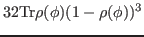
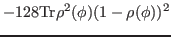
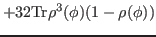
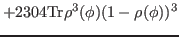
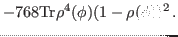
Up to the sixth order, the average Routhian of Eq. (7) to be minimized reads
Average values of powers of the particle-number operator are given in
Eqs. (20)-(25) taken at  . Moreover, in all terms
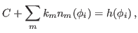
with
. Moreover, in all terms
with  , one can set
  . This gives
Hence, the corresponding mean-field Routhians (to be used in the HFB equations)
reads
1
Although the expression for the mean-field Routhian looks
complicated, it does not require too much of the computational
resources. Additional terms appearing within the Lipkin method are
simply composed by powers of density matrices, and the manipulations
of these terms can be easily performed numerically. The
particle-particle mean fields remain the same, so that the HFB
equations are modified only through Eq. (40).
Lipkin parameters  for
for  can be determined
from Eq. (9) by requiring that it is fulfilled at gauge angle
can be determined
from Eq. (9) by requiring that it is fulfilled at gauge angle  and also at all
  other nonzero values of the gauge angle
  . This gives
 |
|
|
(40) |
where is the flattened Routhian.
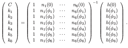
Then, at sixth order, Lipkin parameters  can be easily obtained by inverting the matrix built
of coefficients
can be easily obtained by inverting the matrix built
of coefficients  as
as
At lower orders, or when neglecting odd orders,
a smaller number of the gauge angle points can be used.
In fact, the value of obtained from the first row of
Eq. (42) does not appear in the mean-field Routhian
(40) and can be ignored. Anyhow, at convergence it is
calculated from Eq. (39). Moreover, during the iteration of
the HFB equation, parameter
 is treated as a
Lagrange multiplier, determined so as to adjust the average
particle number, for which, at convergence, one has
is treated as a
Lagrange multiplier, determined so as to adjust the average
particle number, for which, at convergence, one has
 and thus
  has no influence on the value of the right-hand side
of Eq. (39). It means that in the linear
equation (41), the term related to can be simply moved
from the left hand side to the right, and the dimension of the matrix
in Eq. (42) can be further reduced correspondingly.
has no influence on the value of the right-hand side
of Eq. (39). It means that in the linear
equation (41), the term related to can be simply moved
from the left hand side to the right, and the dimension of the matrix
in Eq. (42) can be further reduced correspondingly.
Jacek Dobaczewski
2014-12-07