In the HFB theory with the zero-range
Skyrme interaction [168,169],
or in the local density approximation (LDA) (cf. Refs. [170,167]), the energy functional depends only on local
densities, and on local densities built from derivatives up to the
second order. These local densities are obtained by setting
![]() =
=
![]() in Eqs. (20)-(26) after the derivatives are performed. They will be denoted by having
one spatial argument to distinguish them from the non-local densities
that have two. Moreover, for local densities the spatial argument
will often be omitted in order to lighten the notation.
in Eqs. (20)-(26) after the derivatives are performed. They will be denoted by having
one spatial argument to distinguish them from the non-local densities
that have two. Moreover, for local densities the spatial argument
will often be omitted in order to lighten the notation.
Following the standard definitions [171,172], a number of local densities are introduced:
![]() scalar densities:
scalar densities:
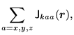
![]() vector densities:
vector densities:
![]() tensor densities:
tensor densities:
We note here in passing that the complete list of all local densities
(up to the derivatives of the second order) also includes the kinetic
and spin-kinetic densities in which the two derivatives are coupled
to a tensor, i.e.,
![]()
![]()
![]() . The
resulting local densities are usually disregarded, because they do not
have counterparts to form useful terms in the local energy density.
There is one set of exceptions, which has been overlooked in the
systematic construction presented in Ref. [173], and
appears in the averaging of a zero-range tensor force [171],
namely, the set of the tensor-kinetic local densities
(48). In Sec. 4 we define terms in
the energy density that depend on the tensor-kinetic densities.
. The
resulting local densities are usually disregarded, because they do not
have counterparts to form useful terms in the local energy density.
There is one set of exceptions, which has been overlooked in the
systematic construction presented in Ref. [173], and
appears in the averaging of a zero-range tensor force [171],
namely, the set of the tensor-kinetic local densities
(48). In Sec. 4 we define terms in
the energy density that depend on the tensor-kinetic densities.
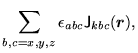
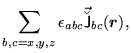
All tensor densities (50) can be decomposed into trace,
antisymmetric, and symmetric parts, giving the standard pseudoscalar,
vector, and pseudotensor components that we show here to fix the
notation:
It follows from Eqs. (28) and (34) that the p-h densities are all real whereas the p-p densities are in general complex and thus the complex-conjugate densities are relevant. The p-p densities become real or imaginary only when the time-reversal symmetry is conserved, see Sec. 7.
Instead of the isoscalar and the third component of isovector
p-h density
one can always use the neutron and the proton one, e.g.,