The HFB sum rules derived in Sec. 2.3 are based on the linearity of the Hamiltonian, by which a matrix element involving the HFB state is a sum of matrix elements calculated for all the PNP components (18). In order to derive the analogous sum rules for the projected DFT energies, one can only use properties of the underlying transition energy density. To this end, we recall that in the HFB theory, the mixing of particle numbers corresponds to the broken U(1) gauge symmetry, and that the PNP actually corresponds to expanding the HFB state in irreducible representations of this group. This observation can be extended to the DFT transition energy density, expanded in these same irreducible representations, with the projected DFT energies being the expansion coefficients. The resulting sum rules must follow from the closure relations on the group manifold.
These general remarks can be expressed in an explicit form in the
following way. By using integration contours that are circles of
radius ![]() around the origin,
around the origin,
![]() , we have the
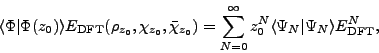
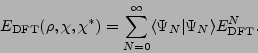
following expression for the projected DFT energy (34)
, we have the
following expression for the projected DFT energy (34)
We note that in the above derivations, ![]() is an arbitrary complex
number; its modulus fixes the radius of integration contour, while its phase
gives the point on the circle that fixes the starting point of the
integral in Eq. (48). This starting point has obviously no
importance for the value of the integral. The sum rule (50)
gives, therefore, a representation of the DFT transition energy density in
terms of a series expansion in
is an arbitrary complex
number; its modulus fixes the radius of integration contour, while its phase
gives the point on the circle that fixes the starting point of the
integral in Eq. (48). This starting point has obviously no
importance for the value of the integral. The sum rule (50)
gives, therefore, a representation of the DFT transition energy density in
terms of a series expansion in ![]() , which converges only on the
ring between the poles. For each such ring, the projected DFT energies
, which converges only on the
ring between the poles. For each such ring, the projected DFT energies
![]() are different, and the DFT transition energy density is
thus equal to a different series expansion. It is obvious that
these different values of the projected DFT energies do not
contradict the continuity of the DFT transition energy density. In this way,
all projected DFT energies for arbitrarily chosen contours of
integration correspond to this same common DFT energy functional.
are different, and the DFT transition energy density is
thus equal to a different series expansion. It is obvious that
these different values of the projected DFT energies do not
contradict the continuity of the DFT transition energy density. In this way,
all projected DFT energies for arbitrarily chosen contours of
integration correspond to this same common DFT energy functional.