


Next: The DFT sum rules
Up: Particle-Number-Projected DFT
Previous: Analytic properties
Residues
Let us now discuss the residues of the integrand
(35). From Eqs. (25) and (33), we see
that the integrand is an odd function of  ,
,
 |
(36) |
This is obvious for even particle numbers  , for which Eq. (25)
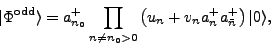
has been derived, while for odd , an additional power
of appears when shifting the blocked HFB state,
, for which Eq. (25)
has been derived, while for odd , an additional power
of appears when shifting the blocked HFB state,
 |
(37) |
i.e.,
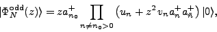 |
(38) |
which gives
 |
(39) |
and renders the integrand (35) an odd function of
also for odd systems.
Near the pole (28), the term in the integrand that produces the residue
has the structure:
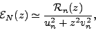 |
(40) |
where
 is an odd function of , regular at the pole.
Similarly, for the pole at =0 we have
is an odd function of , regular at the pole.
Similarly, for the pole at =0 we have
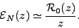 |
(41) |
Therefore, for pairs of poles that are symmetric with
respect to =0, the residues,
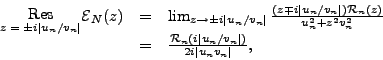 |
(42) |
have identical values. Hence, poles below and above the real axis
yield the same contribution to the contour integral. Based on this
consideration, the projected DFT energy (34), expressed in
terms of residues, reads:
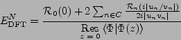 |
(43) |
or
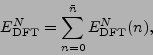 |
(44) |
where
 denotes the contribution from the
  th
pole, including the =0 pole at the origin
up to
th
pole, including the =0 pole at the origin
up to  (last pole encircled by
  ).
).
As an example, we explicitly calculate the residues for a term
that depends on the squared
particle density,
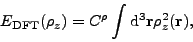 |
(45) |
with
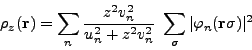 |
(46) |
and  being a coupling constant.
Assuming a two-fold Kramers degeneracy,
the corresponding residue at
being a coupling constant.
Assuming a two-fold Kramers degeneracy,
the corresponding residue at
 is:
is:
 |
(47) |
One can see that residues can be very large for poles
corresponding to canonical states that have occupation numbers close to 1.
These very large contributions to the projected DFT energy must be
compensated by a similarly large contribution from the single pole at
=0. Therefore, within the DFT formalism,
one cannot use the HFB expression (15)
that involves only one residue at =0.
Recall from our discussion in Sec. 3.3
that the poles have the order of  .
In the above example,
the polynomial order is
.
In the above example,
the polynomial order is  =2; hence, the residue (47)
must vanish if the degeneracy
factor
=2; hence, the residue (47)
must vanish if the degeneracy
factor  . This is indeed the case
as for
. This is indeed the case
as for 
 for at least one value of
  .
.
Next: The DFT sum rules
Up: Particle-Number-Projected DFT
Previous: Analytic properties
Jacek Dobaczewski
2007-08-08