


Next: Dependence of projected energy
Up: Numerical examples
Previous: Numerical examples
Numerical accuracy
To calculate residues,
we take circular contour integrals of radius  :
:
 |
(53) |
The integrals are evaluated
using the Fomenko discretization method [42,43],
whereby values of integrands are summed up at gauge angles
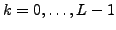
 for
for
 . This corresponds to the
upper half circle in the complex
. This corresponds to the
upper half circle in the complex  -plane
and, as discussed in Sec. 3.2, only the real part of
the integral is kept. For analytic integrands, the Fomenko method
delivers exact results up to admixtures of wave functions with
-plane
and, as discussed in Sec. 3.2, only the real part of
the integral is kept. For analytic integrands, the Fomenko method
delivers exact results up to admixtures of wave functions with
 particles. The main question in
applying this method to non-analytic integrands, which have poles in
the complex plane, is to what extend can it deliver equally accurate
numerical results.
particles. The main question in
applying this method to non-analytic integrands, which have poles in
the complex plane, is to what extend can it deliver equally accurate
numerical results.
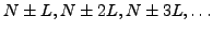
The Fomenko method clearly fails when there is a pole (28)
lying just on the integration contour,  , and an even number of
points
, and an even number of
points  is used. In such a case, the
integration point with
is used. In such a case, the
integration point with  =
= is located exactly at the pole of the integrand. Therefore,
in most practical calculations, an odd number of integration points,
most often
is located exactly at the pole of the integrand. Therefore,
in most practical calculations, an odd number of integration points,
most often  or 9, was used.
However, a more stringent condition on
results from the fact that the discretization method must fail
whenever the integrand varies too rapidly between two neighboring integration points.
Therefore, the spacing between points  must be appropriately
smaller than the distance from the pole. For odd values of , the integration
points corresponding to
must be appropriately
smaller than the distance from the pole. For odd values of , the integration
points corresponding to 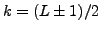 are closest
to the imaginary axis; hence, one arrives at the condition
are closest
to the imaginary axis; hence, one arrives at the condition
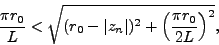 |
(54) |
or
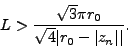 |
(55) |
In the present study, a large number of  integration points
was used, which allows for calculating the contour integrals with
radii that differ by as little as 3% from the position
of the closest pole
integration points
was used, which allows for calculating the contour integrals with
radii that differ by as little as 3% from the position
of the closest pole  .
.
Next: Dependence of projected energy
Up: Numerical examples
Previous: Numerical examples
Jacek Dobaczewski
2007-08-08