Dependence of projected energy on integration contours in spherical nuclei

Table: Contributions $E^N_{\mbox{\rm\scriptsize{DFT}}}(n)$ in $^{18}$O from the individual neutron poles to the projected DFT energy (44) for $N=10$ calculated using the SIII and SLy4 Skyrme functionals. For each parametrization, the last column shows the sum of the $n$th lowest contributions (44), with the values of $E^N_{\mbox{\rm\scriptsize{DFT}}}$ marked by boxed numbers. Canonical energies $\epsilon _n$ and pole positions $z_n$ are also given. All energies are in MeV.

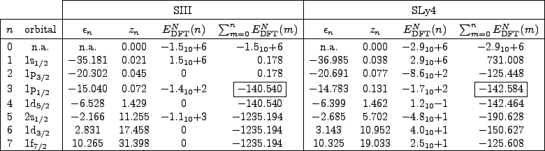
Table 1 displays the results of PNP calculations performed for $^{18}$O by using circular integration contours (53) of different radii. The precision of numerical integrations was confirmed by calculating contributions from individual poles. This was done by carrying out contour integrals over small circles surrounding the poles. In this way, we determined residues from the individual poles $E^N_{\mbox{\rm\scriptsize {DFT}}}(n)$ and checked that their sums, $\sum_{m=0}^nE^N_{\mbox{\rm\scriptsize {DFT}}}(m)$, agree very well with the results of contour integrals along circular contours $C$, as required by the Cauchy theorem (44).

Figure 6: (color online) The $N=10$ projected DFT-SLy4 energies (44) calculated in $^{18}$O as functions of the integration radius $r_0$. Upper (a) and lower (b) panels show, respectively, results for the terms originating from density-independent and density-dependent parts of the Skyrme force. Positions of individual neutron poles are marked by arrows. The inset shows the results near the 2s$_{1/2}$ pole on an expanded scale. The result of calculations obtained with the equivalent contours passing below the branching point associated with the 2s$_{1/2}$ pole (cf. Fig. 5) is shown by a dotted line.

As seen in Table 1, contributions of the $n=0$ poles at $z=0$ are huge. Therefore, the DFT residues at $z=0$ cannot at all be interpreted as the projected energies, as was the case for the PNP HFB theory, Eq. (15). Residues at $z=0$ are cancelled, to a large extent, by contributions from the 1s$_{1/2}$ deep-hole states, which are large because they contain large factors of the type $\left(-{v_n^2}/{u_n^2}\right)^{N}$ for $u_n^2\simeq0$ [see Eq. (47]. Contributions from other poles are also quite large, and apart from the integration contour at $\vert z\vert=1$, none of the other contours reproduce the correct projected energy shown by a boxed number.

For the SIII parametrization, one can see that contributions from poles associated with spherical states with $j\geq 3/2$ ($q \geq 2$) are indeed equal to zero, cf. discussion in Sec. 3.3. This property does not hold for SLy4, for which the projected DFT energies have jumps also when the integration contours cross the $j\geq 3/2$ poles. In this case, the jumps are not related to non-zero residues, but, as discussed in Sec. 3.6, they are caused by the fact that the integration contours are not closed for the fractional-power terms.

Figure 6 shows the projected DFT-SLy4 energies obtained by using circular integration contours of different radii $r_0$. These calculations illustrate properties of poles listed in Table 1. The contributions originating from the density-independent and density-dependent terms of the Skyrme force are separated. The latter terms yield the fractional-power terms in the DFT energy density discussed in Sec. 3.6. As in the SIII case, the density-independent terms exhibit jumps only at the two $j=1/2$ poles. On the other hand, the density-dependent terms show jumps at all poles, and these jumps carry over to the total projected DFT energies shown in Table 1. [The small jump at the 1d$_{5/2}$ pole, 120keV, is practically invisible in the scale of Fig. 6.] Moreover, contributions of the density-dependent terms are not constant between the poles, as would be required by the Cauchy theorem. This is caused by the prescription (52) to step over the cuts in the complex plane, and illustrates spurious contributions to the projected DFT energies discussed in Sec. 3.6. As shown in the blown-up inset in Fig. 6(b), these spurious contributions appear just below the pole thresholds (i.e., for small negative values of $r_0-\vert z_n\vert$), and they can be quite large - of the order of several tens of MeV. The gradual development of spurious contributions below threshold has been explained in Sec. 3.6. Namely, if the contour radius is only slightly greater than $\vert z_{n-1}\vert$, the branching point associated with the pole $z_n$ is always outside for all values of $\bf r$. With increasing $r_0$, more and more branching points corresponding to different regions of space fall inside the contour, leading to the spurious behavior. As discussed earlier, one can eliminate this subthreshold effect by taking equivalent contours discussed in the context of Fig. 5. Such a procedure is illustrated by a dotted line in the inset of Fig. 6(b).

The spurious contributions may result in large errors in the projected PNP energies, making results of the standard PNP calculations meaningless. Unfortunately, this is true not only for Skyrme forces that use density-dependent terms of fractional orders but also for the Gogny force, which contains a density-dependent term of order $\gamma=1/3$.