Models of structure of the Sn isotopes

In the present study, the properties of even-even Sn isotopes (masses 100 to 176) are described using the spherical mean-field Hartree-Fock-Bogoliubov (HFB) model [12]. Two Skyrme interactions have been used. As a description of the method has been given in detail elsewhere [19,20,14]; only details pertaining to the particular calculations made and used herein are given. We have used two parameterizations of the Skyrme force, SkP [19] and SLy4 [21], that are known to give a correct description of bulk nuclear properties. They differ by the input values of the nuclear-matter effective mass, being m^*/m = 1 and 0.7 respectively. The zero-range density-dependent pairing force was used in the particle-particle channel, with the form that is intermediate between volume and surface attraction [14]. A large positive energy phase space of 60 MeV was taken and for which the pairing-force strengths of V₀=-286.20 and -212.94 MeV fm^-3 were obtained in the SkP and SLy4 cases respectively. Those strengths result on using a standard adjustment [22] of the neutron pairing gap in ¹²⁰Sn.

  

Figure 1: Two-neutron separation energies S_2N(lower) and the neutron pairing gaps $\Delta_N$ (upper) obtained within the HFB/SkP and HFB/SLy4 models compared with experimental data.

In Fig. 1 we compare with data, the two-neutron separation energies S_2N and the neutron pairing gaps $\Delta_N$ calculated from the two HFB models so that the quality of the description of the Sn isotopes may be judged. Experimental pairing gaps of even-Nisotopes were estimated from the nuclear masses [23] as averages $\left[ \Delta^{(3)}\left( N-1 \right) + \Delta^{(3)}\left( N+1 \right) \right]/2$ of the three-point staggering parameters [24] centered at odd neutron numbers (N-1) and (N+1). Evidently a fairly good description of pairing properties is obtained in between the magic numbers N=50 and N=82. At the magic numbers, the calculated gaps vanish due to the known effect of an unphysical, too sudden, pairing phase transition. The size of the jump of S_2Nat N=82 is slightly underestimated (overestimated) by the HFB/SkP (SLy4) model. That is an effect of the different values of the effective mass. Nevertheless, the overall quality of agreement between theory and experiment suffices for us to consider the two models to be useful for extrapolations to describe unknown heavy Sn isotopes.

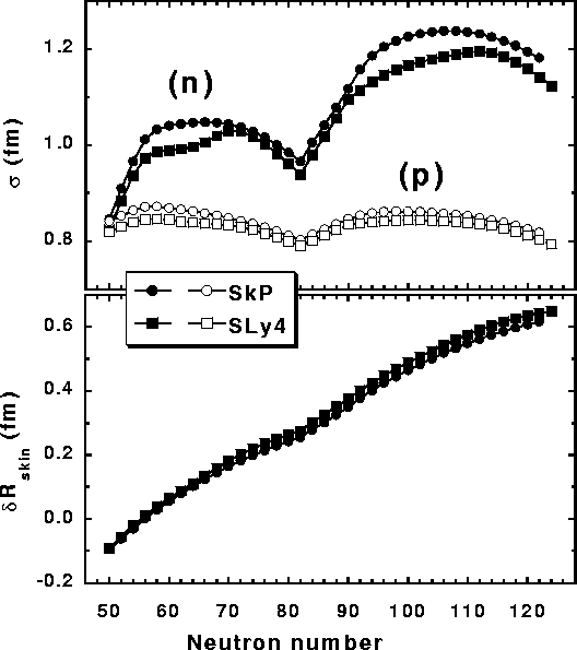
Spatial properties of neutron and proton density distributions are of special interest in a number of contexts. With structure studies, geometric aspects have been found in the past [6] by using the Helm model. Using those methods, four quantities are summarized in Figs. 2 and 3. Results are shown for all even

  

Figure 2: Calculated neutron (filled symbols) and proton (open symbols) diffraction radii (lower) and bulk densities (upper). Circles and squares correspond to the results obtained within the HFB/SkP and HFB/SLy4 models respectively.

  

Figure 3: Same as in Fig. 2, but for the neutron skins (lower) and surface thicknesses (upper).

Sn isotopes between N=50 and the two-neutron drip line (N=122 and N=124 for SkP and SLy4, respectively). These presentations are of the bulk (interior) particle density, $\rho_{\mbox{\rm\scriptsize {bulk}}}$, the diffraction radius, R₀, the surface thickness, $\sigma$, and neutron skin thickness, $\delta{R}_{\mbox{\rm\scriptsize {skin}}}$, as often sought from the microscopically calculated densities $\rho(r)$. R₀ and $\sigma$were obtained by comparing positions of the first zero and first maximum of the microscopic and Helm model form factors. The neutron skin thickness is identified as the difference between neutron and proton Helm radii, $R_{\mbox{\rm\scriptsize {Helm}}} = \sqrt{R_0^2+5\sigma^2}$. Finally, $\rho_{\mbox{\rm\scriptsize {bulk}}}$ was obtained by calculating the average microscopic density $\langle\rho\rangle = 4\pi\int{r}^2\rho^2(r)/A$, and identifying it with the analogous value for the Helm model density in which $\rho_{\mbox{\rm\scriptsize {bulk}}}$ is a parameter.

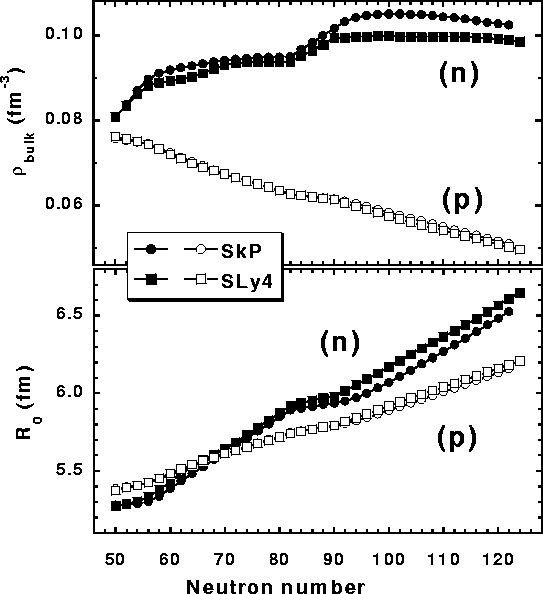Certain features of the calculated HFB neutron and proton densities in the Sn isotopes are readily apparent in these figures. With increasing number of neutrons, the neutron and proton radii increase at different rates; the neutron radii being the faster. As a result there is a gradual increase in the size of the neutron skin; an increase that is almost linear with neutron number. At the same time the neutron and proton bulk densities increase and decrease, respectively. The balance between the bulk and surface increase of the neutron distribution is governed by the volume and surface attractions between neutrons and protons and hence is fixed by the principal features of the volume and surface terms in nuclear masses. Since these are rigidly adjusted to experimental data, the net results obtained with both Skyrme interactions, as expected, are quite similar. Note also from Fig. 3, that the surface thickness of the neutron distributions defined in this way increases by about 50% across the nuclear chart while that of protons stays almost constant, apart from very visible shell fluctuations created by the analogous effects in the neutrons.

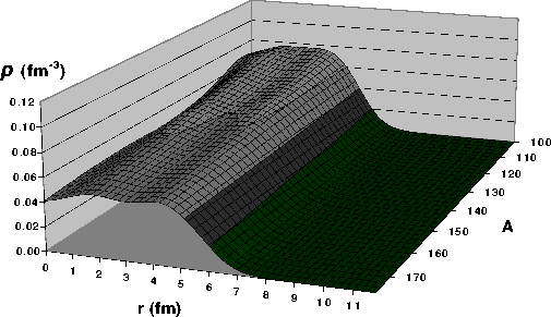
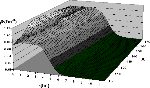
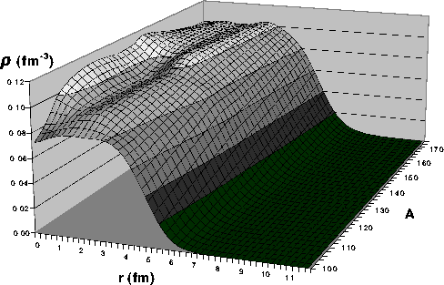
Alternative to the above approach is inspection of the actual density profiles deduced from the shell occupancies and associate canonical wave functions of the mean-field model results. Such complete density distributions for all of the even mass Sn isotopes resulting from the SLy4 and SkP models of their structure are so shown in Figs. 4 through 9.

  

Figure 4: The proton density mass variation from the SLy4 model of structure for the Sn isotopes.

  

Figure 5: The neutron density mass variation from the SLy4 model of structure for the Sn isotopes.

  

Figure 6: The proton density mass variation from the SkP model of structure for the Sn isotopes.

  

Figure 7: The neutron density mass variation from the SkP model of structure for the Sn isotopes.

  

Figure 8: The proton densities given by the SLy4 model of structure for 8 isotopes of Sn.

  

Figure 9: The neutron densities given by the SLy4 model of structure for 8 isotopes of Sn.

Using the SLy4 force, the proton and neutron matter distributions for all even mass Sn isotopes resulting from the mean-field calculations are displayed in Figs. 4 and 5 respectively. The proton (neutron) distributions are plotted with nuclear mass decreasing (increasing) into the page. By that means the variations to those densities are best portrayed in block form. The proton number of course is fixed at 50 and so as the neutron number increases, and concomitantly the neutron volume increases, those 50 protons extend over an increasing volume. As noted above that is due to the strong attractive neutron-proton interactions. In concert, the central charge density must, and does, decrease. However, and as will be seen more clearly in Fig. 8 below, the charge distributions do not become significantly more diffuse. The prime effect is the $\sim 33\%$ increase in the charge volume.

The neutron densities generated using the SLy4 model have a different structure variation with increasing mass. The general trend that the neutron rms radii increase is evident as the half central density is reached at radii ranging from $\sim 5$ fm in ¹⁰⁰Sn to $\sim 6.5$ fm for ¹⁷⁰Sn. The increase of the neutron surface diffuseness is difficult to see from a direct inspection of the density profiles, although it is evident in the results shown in Fig. 3. We note also that a strong oscillation develops in the central density, which on average also increases from $\sim 0.08$ neutrons/fm³ in ¹⁰⁰Sn to $\sim 0.1$ neutrons/fm³for ¹⁷⁰Sn.

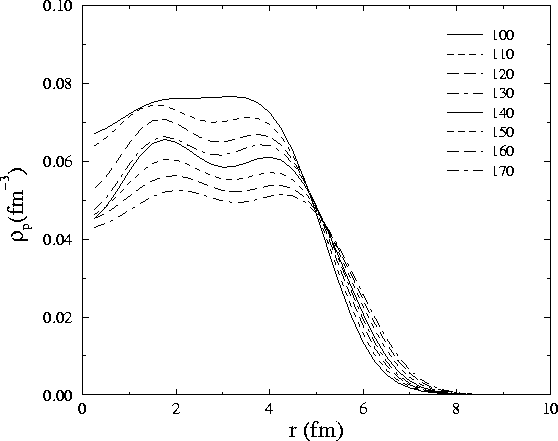
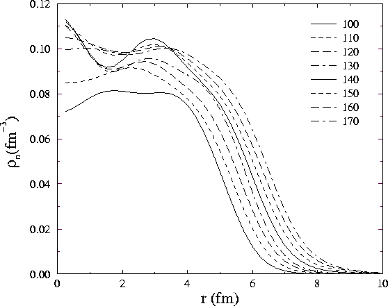
The features identified above also are evident in the results found using the SkP force in the HFB calculations. Those results are shown in Figs. 6 and 7 for the protons and neutrons respectively. Again, for clarity, the proton distributions are plotted with mass decreasing into the page. While the prime features of these densities are as observed with the SLy4 model results, there are differences in detail.

The mass variations of densities are evident also in Figs. 8 and  9 wherein the proton and neutron densities respectively for the Sn isotopes calculated using the SLy4 model are given for a select set of 8 nuclei having masses spaced evenly between 100 and 170. In Fig. 8 it is evident that the 50 protons are rearranged to be more extensive as one increases mass. Note that the half-density radius ranges from $\sim 5$ fm for ¹⁰⁰Sn to $\sim 6$ fm in ¹⁷⁰Sn. However the proton surface diffuseness remains essentially unchanged. The distance over which the charge density falls from 90% to 10% of its central value is $\sim 2$ fm in all nuclei. That is also the case for the neutron distributions. There is a gradual development of a neutron skin to the Sn isotopes, for while with ¹⁰⁰Sn the 50 protons and 50 neutrons have essentially the same distribution (solid dark lines in the figures), the two density profiles are somewhat disparate in ¹⁷⁰Sn. Not only does the neutron central density increase by $\sim 25\%$ from its value in ¹⁰⁰Sn while the proton central density value decreases by $\sim 40\%$, but the skin, in this case $R_{rms}\mbox{\rm\scriptsize {(neutron)}} - R_{rms}\mbox{\rm\scriptsize {(proton)}}$, varies from 0 to $\sim 0.5$ fm as noted previously from the definition in the Helm model characterization.