Iterative solution of the RPA equations

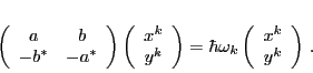
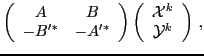
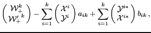
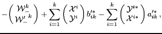
The RPA equations (3) and (4) constitute a non-hermitian eigenproblem with non-positive-definite norm. We solve this problem by using an iterative method that during each iteration only needs to know the product of the RPA matrix and a density vector, that is, the right-hand sides of Eqs. (3) and (4):

$$W^k_{mi} = \left(\epsilon_m-\epsilon_i\right) X_{mi}^k + {\tilde h}_{mi}({\mathcal X}^k,{\mathcal Y}^k) \,,$$ (6)

$$W'^k_{mi} = \left(\epsilon_i-\epsilon_m\right) Y_{mi}^k - {\tilde h}_{im}({\mathcal X}^k,{\mathcal Y}^k) \,,$$ (7)

where index $k$ labels iterations and the mean fields ${\tilde h}({\mathcal X}^k,{\mathcal Y}^k)$ depend linearly on the density vectors ${\mathcal X}^k$ and ${\mathcal Y}^k$. Expressed through the standard RPA matrices $A$ and $B$ [12], Eqs. (6) and (7) for a positive norm basis vector and for its opposite norm partner vector read:

$$\left( \begin{array}{c} {\mathcal W}_+^k\\ {{\mathcal W}'_+}^k\\ \end{array} \right) = \left( \begin{array}{cc} A & B \\ -B'^* & -A'^* \\ \end{a... ...{array}{c} {{\mathcal X}}^k \\ {{\mathcal Y}}^k \\ \end{array}\right)\,,$$ (8)

$$\left( \begin{array}{c} {\mathcal W}_-^k\\ {{\mathcal W}'_-}^k\\ \end{array} \right) = \left( \begin{array}{cc} A & B \\ -B'^* & -A'^* \\ \end{a... ...}{c} {{\mathcal Y}}^{k*} \\ {{\mathcal X}}^{k*} \\ \end{array}\right)\,.$$ (9)

In exact arithmetic $A=A'$ and $B=B'$ and therefore either Eqs. (8) or (9) could be used in the iteration procedure with equivalent results. Nevertheless, below we use them both to stabilize the iteration process.

Various iterative methods, which only need to know the products of the diagonalized matrix and vectors, exist for non-hermitian matrix eigenvalue equations, and good examples with pseudocode are shown in Ref. [1]. We chose the non-hermitian Lanczos method [5] in a modified form, because it conserves all odd-power energy weighed sum rules (EWSR) if the starting vector (pivot) of iteration is chosen correctly. 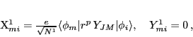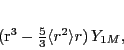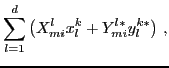In this work, we start from a pivot vector that has its elements set to the matrix elements of electromagnetic multipole operator,

$${X}_{mi}^{1} = \frac{e}{\sqrt{N^1}} \langle \phi_m\vert r^p\,Y_{JM} \vert \phi_i\rangle , \quad {Y}_{mi}^{1} = 0\,,$$ (10)

where $p=2$ and $J=0$ for the $0^+$ mode, $p=1$ and $J=1$ for the $1^-$ mode, and $p=2$ and $J=2$ for the $2^+$ mode. The constant $N^1$ is used to normalize the pivot vector to unity. For the IS $1^-$ mode we only present results obtained with the operator:

$$(r^3 - {\textstyle{5\over 3}} \langle r^2\rangle r)\,Y_{1M},$$ (11)

to stay consistent with Refs. [16] and [17]. For the choice of pivot in (10) one can prove [5] that all odd-power EWSRs are satisfied throughout the iteration procedure.

Because we calculate the RPA matrix-vector products by using the mean-field method, and not with a precalculated RPA matrix, we introduce small, but significant numerical noise to the resulting vectors. If corrective measures are not used to remove or reduce this noise, the iteration method fails and produces complex RPA eigenvalues early on in the iteration. We stabilize our iterative solution method by modifying the method of Ref. [5] in two ways. First, we use the non-hermitian Arnoldi method instead of the non-hermitian Lanczos method. 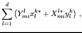The advantage of Arnoldi method is that it orthogonalizes each new basis vector against all previous basis vectors and their opposite norm partners, that is,

$$\left(\!\! \begin{array}{c} {\tilde{\mathcal X}}^{k+1} \\ {\tilde{\mathcal Y}}^{k+1} \\ \end{array} \!\!\right) =\!\! \left(\!\! \begin{array}{c} {\mathcal W}_+^k \\ {{\mathcal W... ...al Y}}^{i*} \\ {{\mathcal X}}^{i*} \\ \end{array} \!\!\right) b_{ik} \,,$$ (12)

$$\left(\!\! \begin{array}{c} {\tilde{\mathcal Y}}^{k+1*} \\ {\tilde{\mathcal X}}^{k+1*} \\ \end{array} \!\!\right) =\!\! -\!\left(\!\! \begin{array}{c} {\mathcal W}_-^k \\ {{\mathca... ... Y}}^{i*} \\ {{\mathcal X}}^{i*} \\ \end{array} \!\!\right) a'^*_{ik}\,,$$

where the overlap matrices $a_{ik}$, $b_{ik}$, $a'^*_{ik}$, and $b'^*_{ik}$ are calculated as in Eq. (5). Again, in exact arithmetic, Eqs. (12) and (13) are equivalent and the lower matrix elements $a'^*_{ik}$ and $b'^*_{ik}$ in Eq. (13) are exact complex conjugates of the elements of the upper Krylov-space [18] RPA matrices. We assume this to keep the Krylov-space RPA matrix in the standard form.

In the Lanczos method, only the tridiagonal parts of RPA matrices are calculated, and small changes in basis vectors due to Lanczos re-orthogonalization (which always must be used to preserve orthogonality) do not show up in the constructed RPA matrix. In the Arnoldi method, these small but important elements outside the tridigonal part improve the stability as compared to Lanczos.

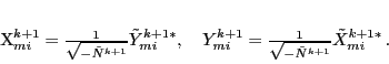
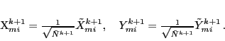
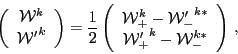
The norm of the obtained new residual vector in Eq. (12) can be either positive or negative. We do not in practice use Eq. (13), which in exact arithmetic would duplicate the results of Eq. (12). Instead, we store only the positive-norm basis states and use a similar method as in Ref. [5] to change sign of the norm in case the norm of the residual vector in Eq. (12) is negative. Thus, explicitly, for the positive norm of the residual vector $\tilde{N}^{k+1} = \langle \tilde{X}^{k+1},\tilde{Y}^{k+1}\vert \tilde{X}^{k+1},\tilde{Y}^{k+1} \rangle$, we define the new normalized positive-norm basis vector as

$${X}_{mi}^{k+1} = \frac{1}{\sqrt{\tilde{N}^{k+1}}} \tilde{... ...+1} = \frac{1}{\sqrt{\tilde{N}^{k+1}}} \tilde{Y}_{mi}^{k+1}\,.$$ (13)

If $\tilde{N}^{k+1}<0$, the new normalized positive norm basis vector is defined as

$${X}_{mi}^{k+1} = \frac{1}{\sqrt{-\tilde{N}^{k+1}}} \tilde... ...} = \frac{1}{\sqrt{-\tilde{N}^{k+1}}} \tilde{X}_{mi}^{k+1*}\,.$$ (14)

When maximum number of iterations has been made or the iteration has been stopped, the generated Krylov-space RPA matrix, with dimension $d << D$, is diagonalized with standard methods, that is we solve:

$$\left( \begin{array}{cc} a & b \\ -b^* & -a^* \\ \en... ...in{array}{c} {x}^{k} \\ {y}^{k} \\ \end{array} \right)\,.$$ (15)

The approximate RPA solutions are then obtained by transforming the Krylov-space basis vectors,

$$X^k_{mi} = \sum_{l=1}^d \left( {X}^l_{mi} x_{l}^k + {Y}^{l*}_{mi}y_{l}^{k*}\right)\,,$$ (16)

$$Y^k_{mi} = \sum_{l=1}^d \left( {Y}^l_{mi} x_{l}^{k*} + {X}^{l*}_{mi} y_{l}^{k}\right)\,,$$ (17)

for all $k=1,\ldots,d$, and these vectors are used to evaluate the strength functions.

Standard RPA method that constructs and diagonalizes the full RPA matrix can ensure that the lower matrices in the RPA supermatrix are exact complex conjugates of the upper matrices. Our mean-field method can have small differences in the implicitly used upper and lower RPA matrices due to finite numerical precision. The consequence of this is that we will in general have $a'_{ij} \neq a_{ij}$ and $b'_{ij} \neq b_{ij}$. This spoils the consistency of Eqs. (12) and (13) and can make the Arnoldi iteration to fail and produce complex energy solutions.

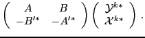
The numerical errors in the matrix-vector products can be reduced by symmetrization. We thus calculate the RPA fields twice, first using the densities of a positive norm basis vector $( {{\mathcal X}}^k, {{\mathcal Y}}^k)$, and second using the densities of negative norm vector $( {{\mathcal Y}}^{k*}, {{\mathcal X}}^{k*})$. The two resulting vectors are subtracted from each other to get the final stabilized RPA matrix-vector product,

$$\left( \begin{array}{c} {\mathcal W}^k\\ {{\mathcal W}'}... ...cal W}'_+}^k - {\mathcal W}_-^{k*}\\ \end{array} \right) \,,$$ (18)

to be used in Eq. (12). Together, the Arnoldi iteration method and symmetrization of matrix-vector products stabilize our mean-field based iterative diagonalization.