Treatment of spurious RPA modes

For the discussion of various spurious modes in the RPA method we refer the reader to, e.g., Ref. [13]. In the present study, we only consider spherical ground states neglecting pairing correlations, so the only spurious excitation is generated by the total linear momentum. Therefore, the only affected RPA mode is the isoscalar $1^-$ mode. In traditional RPA calculations that construct and diagonalize the full RPA matrix, the spurious $1^-$ mode is typically removed after the RPA diagonalization. Often a modified transition operator (11) is used, which has the property of $\langle HF\vert \left[ {\hat F}, {\hat P}_{cm}\right]\vert HF\rangle =0$, as long as the commutator is evaluated within a complete set of basis states. In a finite model spaces of localized orbitals this relation is no more exactly valid, and the corrected operator does not remove spurious components exactly.

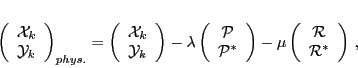
To remove the spurious isoscalar $1^-$ mode from our physical RPA excitations we use the same method as in Ref. [6], where the basis vectors are orthogonalized against the spurious translational mode ${\mathbf P}$ and its conjugate "boost" operator ${\mathbf R}$, which have the form:

$${\hat P}_{\mu} = \frac{1}{\sqrt{3}} \sum_{mi} \left( i( \phi_m\vert\vert \nabla_1\... ..._i) \left[c^\dagger _{m}\tilde c^{ }_{i}\right]_{1\mu} + {\rm h.c.} \right)\,,$$ (19)

$${\hat R}_{\mu} = \frac{1}{\sqrt{3}} \sum_{mi} \left( ( \phi_m\vert\vert r_1\vert\v... ..._i) \left[c^\dagger _{m}\tilde c^{ }_{i}\right]_{1\mu} + {\rm h.c.} \right)\,.$$ (20)

The spurious RPA vectors $({\mathcal P}, {\mathcal P}^*)$ and $({\mathcal R}, {\mathcal R}^*)$ contain the p-h and h-p matrix elements of Eqs. (20) and (21), respectively. Our method differs from that of Ref. [6] in the fact that we orthogonalize our basis during the Arnoldi iteration, which fits naturally with the iterative solution method and guarantees that the obtained approximate RPA excitations have exact zero overlaps with spurious modes. This is equivalent to diagonalizing the full RPA matrix in the subspace orthogonal to the spurious states. In our implementation, each generated new Arnoldi basis vector is orthogonalized as

$$\left( \begin{array}{c} {{\mathcal X}}_k \\ {{\mathca... ...{\mathcal R} \\ {\mathcal R}^* \\ \end{array} \right) \,,$$ (21)

where the overlaps $\lambda$ and $\mu$ are defined as

$$\lambda = \frac{\langle R,R^*\vert {X}^k,{Y}^k \rangle }{\langle R,R^*\vert P,P^* \rangle }\,,$$ (22)

$$\mu = -\frac{\langle P,P^*\vert {X}^k,{Y}^k \rangle }{\langle R,R^*\vert P,P^* \rangle }\,.$$ (23)

When more symmetries are broken, formulas equivalent to Eqs. (22)-(24) can be used to remove spurious components coming from each broken symmetry of the mean field.