The regression coefficients ![]() obtained in the present work
can be used to evaluate the possibility of readjusting the EDF coupling
constants so as to better describe the experimental data. Indeed,
if for a given set of coupling constants
obtained in the present work
can be used to evaluate the possibility of readjusting the EDF coupling
constants so as to better describe the experimental data. Indeed,
if for a given set of coupling constants ![]() the self-consistent
s.p. energies are equal to
the self-consistent
s.p. energies are equal to
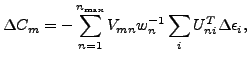
![]() , then corrections to
coupling constants
, then corrections to
coupling constants
![]() are given by:
are given by:
Singular values ![]() obtained for regression coefficients
obtained for regression coefficients
![]() corresponding to three Skyrme functionals are shown in
the lower panel of Fig. 16. Independently of which functional
is concerned, the singular values decrease exponentially from
about 1.3 to 0.001. Again, this illustrates a great universality of
the regression coefficients.
corresponding to three Skyrme functionals are shown in
the lower panel of Fig. 16. Independently of which functional
is concerned, the singular values decrease exponentially from
about 1.3 to 0.001. Again, this illustrates a great universality of
the regression coefficients.
On the one hand, as seen in Eq. (13), small singular values
![]() correspond to columns of matrices
correspond to columns of matrices ![]() and
and ![]() that have
very small influence on the matrix of regression coefficients
that have
very small influence on the matrix of regression coefficients
![]() . On the other hand, these same small singular values
have very large impact on the coupling constants in
Eq. (14). Therefore, expression (14) should be used
for non-maximum values of
. On the other hand, these same small singular values
have very large impact on the coupling constants in
Eq. (14). Therefore, expression (14) should be used
for non-maximum values of
![]() , i.e., by cutting off the
small singular values. By that, one removes from the final result
those features of the regression coefficients that are poorly defined,
and at the same time one keeps only those linear combinations of coupling
constants that are well determined by data.
, i.e., by cutting off the
small singular values. By that, one removes from the final result
those features of the regression coefficients that are poorly defined,
and at the same time one keeps only those linear combinations of coupling
constants that are well determined by data.
![\includegraphics[width=\textwidth]{fig16.eps}](img126.png) |
In our analysis, for experimental data we adopted ![]() proton and neutron
negative s.p. listed in Ref. [20]. Since here we study
bare theoretical s.p. energies, we have also subtracted from
the experimental values the calculated mass polarization corrections related to
the one-body center-of-mass correction [5].
In the upper panel of Fig. 16, we show the rms deviations,
proton and neutron
negative s.p. listed in Ref. [20]. Since here we study
bare theoretical s.p. energies, we have also subtracted from
the experimental values the calculated mass polarization corrections related to
the one-body center-of-mass correction [5].
In the upper panel of Fig. 16, we show the rms deviations,
At this point, we would like to stress that in this study we fit only the s.p. energies, while in reality many other observables should be (and were in the past) included in the fitting procedure. In particular, in Ref. [21] the s.p. energies along with global nuclear properties were used to fit the Skyrme force parameters. However, our results indicate that there exist limiting lower values of the rms deviations (15). By adding other observables to the fit, one can only obtain higher values thereof, i.e., worse descriptions of the s.p. energies.
![\includegraphics[width=\textwidth]{fig17.eps}](img133.png) |
Although in particular cases, some combinations of the coupling
constants are especially important, i.e., at
![]() 7-8
for SkO' or at
7-8
for SkO' or at
![]() 4 for SkP, the rms deviations
decrease rather steadily (especially for SLy5), and do not show pronounced affects at low
values of
4 for SkP, the rms deviations
decrease rather steadily (especially for SLy5), and do not show pronounced affects at low
values of
![]() , observed previously for the total binding
energies, see Fig. 2 in Ref. [9]. On the one hand, this
means that the experimental values of the s.p. energies may, in
principle, determine values of more coupling constants than those of
the total binding energies. On the other hand, the limiting value of
, observed previously for the total binding
energies, see Fig. 2 in Ref. [9]. On the one hand, this
means that the experimental values of the s.p. energies may, in
principle, determine values of more coupling constants than those of
the total binding energies. On the other hand, the limiting value of
![]() 1.1MeV, which can be obtained by
refitting the standard functionals, is rather disappointing.
Fig. 17 shows histograms of residuals, Eq. (12),
for standard (upper panels) and linearly refitted (lower panels) Skyrme
functionals. One can see again that the improvement obtained by the
fit is not very spectacular, with quite a number of s.p. energies
differing from experiment by 1MeV or more. This indicates, that to
obtain a better agreement with experimental one may have to extend
the form of the standard Skyrme functional.
1.1MeV, which can be obtained by
refitting the standard functionals, is rather disappointing.
Fig. 17 shows histograms of residuals, Eq. (12),
for standard (upper panels) and linearly refitted (lower panels) Skyrme
functionals. One can see again that the improvement obtained by the
fit is not very spectacular, with quite a number of s.p. energies
differing from experiment by 1MeV or more. This indicates, that to
obtain a better agreement with experimental one may have to extend
the form of the standard Skyrme functional.