In this section, we review the basic ingredients of Hartree-Fock-Bogoliubov theory and the Lipkin-Nogami method followed by particle-number projection. Since these are by now standard tools in nuclear structure, we keep the presentation brief and refer the reader to Ref. [30] for further details.
HFB is a variational theory that treats in a unified fashion
mean-field and pairing correlations. The HFB equations can be
written in matrix form as
In coordinate representation, the HFB approach consists of solving
(1) as a set of integro-differential equations with
respect to the amplitudes
![]() and
and
![]() , both of which are functions of the position coordinate
, both of which are functions of the position coordinate ![]() . The resulting density matrix and pairing tensor then read
. The resulting density matrix and pairing tensor then read
In the configurational approach, the HFB equations are solved by
matrix diagonalization within a chosen single-particle basis
{
![]() } with appropriate symmetry properties. In
this sense, the amplitudes
} with appropriate symmetry properties. In
this sense, the amplitudes ![]() and
and ![]() entering
Eq. (1) may be thought of as expansion coefficients for
the quasiparticle states in the assumed basis. The nuclear
characteristics of interest are determined from the density matrix
and pairing tensor,
entering
Eq. (1) may be thought of as expansion coefficients for
the quasiparticle states in the assumed basis. The nuclear
characteristics of interest are determined from the density matrix
and pairing tensor,
The results from configuration-space HFB calculations should be
identical to those from the coordinate-space approach when all the
states
![]() from a complete single-particle basis are
taken into account. Of course, this is never possible. In the
presence of truncation, it is essential that the basis produce
rapid convergence, so that reliable results can be obtained within
computational limitations on the number of basis states that can
be included.
from a complete single-particle basis are
taken into account. Of course, this is never possible. In the
presence of truncation, it is essential that the basis produce
rapid convergence, so that reliable results can be obtained within
computational limitations on the number of basis states that can
be included.
The LN method serves as an efficient method for restoring particle number before variation [24]. With only a slight modification of the HFB procedure outlined above, it is possible to obtain a very good approximation for the optimal HFB state, on which exact particle number projection then has to be performed [28,31].
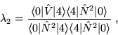
In more detail, the LN method is implemented by performing the HFB
calculations with an additional term included in the HF
hamiltonian,
 |
(9) |
An explicit calculation of ![]() from Eq. (10) requires
calculating new sets of fields Eq. (11),
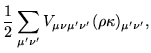
which is rather cumbersome. However, we have found [32]
that Eq. (10) can be well approximated by the seniority-pairing
expression Eq. (13)
with the effective strength
from Eq. (10) requires
calculating new sets of fields Eq. (11),
which is rather cumbersome. However, we have found [32]
that Eq. (10) can be well approximated by the seniority-pairing
expression Eq. (13)
with the effective strength
| (14) |
| (15) |
| (16) |
The use of the LN method in HFB theory requires special consideration
of the asymptotic properties of quasiparticle states
[4,5], of essential importance for weakly-bound
systems. Because of the modified HF hamiltonian (8),
new terms appear in the HFB+LN equation, which are non-local in
coordinate representation and thus can modify the asymptotic
conditions. Effectively, this means that the standard Fermi energy
![]() has to be replaced by
has to be replaced by
The first expression (17) assumes that the asymptotic
properties can be inferred from the HFB equation in the canonical
basis, in which ![]() is diagonal and has eigenvalues that can be
estimated by norms of the second HFB components. The second
expression (18) pertains to the HFB equation in coordinate
representation, in which the integral kernel
is diagonal and has eigenvalues that can be
estimated by norms of the second HFB components. The second
expression (18) pertains to the HFB equation in coordinate
representation, in which the integral kernel
![]() vanishes at large distances. Neither of
these expressions can be rigorously justified, thereby
demonstrating limitations of using the LN method to analyze
spatial properties of wave functions. These ambiguities are
enhanced by the fact that the LN method overestimates the
curvature
vanishes at large distances. Neither of
these expressions can be rigorously justified, thereby
demonstrating limitations of using the LN method to analyze
spatial properties of wave functions. These ambiguities are
enhanced by the fact that the LN method overestimates the
curvature ![]() near magic numbers [28,31].
near magic numbers [28,31].
Note that in the exact projection before variation method, the
Fermi energy is entirely irrelevant, and hence one should not
attribute too much importance to the choice between ![]() and
and
![]() . Nevertheless, since the PNP affects only occupation
numbers, leaving the canonical wave functions unchanged, in what
follows we use the modified Fermi energy
. Nevertheless, since the PNP affects only occupation
numbers, leaving the canonical wave functions unchanged, in what
follows we use the modified Fermi energy ![]() in modelling
the asymptotic behavior needed to implement the THO method.
in modelling
the asymptotic behavior needed to implement the THO method.
Finally, we should note that the HFB machinery detailed above can be readily implemented with a quadrupole constraint [30], as is the case for some of the calculations we will be reporting.