Next: The Lipkin-Nogami method
Up: Variation after particle-number projection
Previous: Variation after particle-number projection
The HFB+VAPNP method
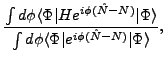
It has been demonstrated [25] that the
HFB+VAPNP energy,
where  is the particle-number projection operator,
 |
(27) |
can be written as an energy functional of the unprojected densities
(7).
The variation of Eq. (26) results in
the HFB+VAPNP equations:
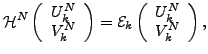 |
(28) |
where
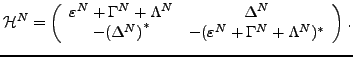 |
(29) |
Equations (28) and (29) have the same structure as
Eqs. (11) and (12), except that the expressions for
the VAPNP fields are now different [25,27], i.e.,
with
where, using the unit matrix  ,
,
 |
 |
 |
(36) |
 |
|
 |
(37) |
 |
|
 |
(38) |
 |
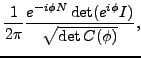
|
![$\displaystyle e^{2i\phi }\left[ 1+\rho (e^{2i\phi }-1)\right]^{-1},$](img126.png) |
(39) |
 |
|
 |
(40) |
 |
|
 |
(41) |
and
After solving the HFB+VAPNP equations (28), one obtains the
intrinsic density matrix and pairing tensor:
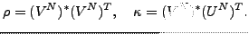 |
(43) |
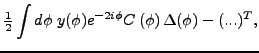
Finally, the total HFB+VAPNP energy is given by
The quantity  plays a role of an
  -dependent metric. The
integrands in Eqs. (30)-(32) take the familiar HFB
limit at
-dependent metric. The
integrands in Eqs. (30)-(32) take the familiar HFB
limit at  =0, while the integrand in (33) vanishes
(
=0, while the integrand in (33) vanishes
(
 does not appear in the standard HFB approach).
Next: The Lipkin-Nogami method
Up: Variation after particle-number projection
Previous: Variation after particle-number projection
Jacek Dobaczewski
2006-10-13

![$\displaystyle \tfrac{1}{2}\int d\phi \,\,y(\phi )\left\{ Y(\phi
){\rm Tr}
[e\rho (\phi )]\right.$](img103.png)
![$\displaystyle \tfrac{1}{4}\int d\phi \,\,y(\phi ) \left\{Y(\phi) {\rm
Tr}
[\Gamma(\phi)\rho(\phi)] \right.$](img106.png)
![$\displaystyle -\tfrac{1}{4}\int d\phi \,\,y(\phi )\left\{ Y(\phi
){\rm Tr}
[\Delta (\phi )\overline{\kappa }^{\ast }(\phi )]\right.$](img111.png)