The Lipkin-Nogami method

The LN method [10,11] constitutes an astute and efficient way of performing an approximate VAPNP calculation. It can be considered [7] as a variant of the second-order Kamlah expansion [8,9], in which the VAPNP energy (26) is approximated by a simple expression,

$$E_{\text{LN}}=E[\rho ,\tilde{\rho}] - \lambda_2(\langle\hat{N}^2\rangle-N^2),$$ (45)

with $\lambda_2$ depending on the HFB state $\vert\Phi\rangle$ and representing the curvature of the VAPNP energy with respect to the particle number. The role of $\lambda_2$ in the Kamlah and LN methods differs. In the former, $\lambda_2$ is varied along with variations of the HFB state $\vert\Phi\rangle$, while in the latter, this variation is neglected. Had the second-order Kamlah expression (45) been exact, the variation of $\lambda_2$ would have been fully justified and the method would be giving the exact VAPNP energy. However, since the second-order expression is, in practical applications, never exact, it is usually more reasonable to adopt the LN philosophy, in which one rather strives to find the best estimate of the curvature $\lambda_2$ instead of finding it variationally in an approximate way.

When the HFB method is applied to a given Hamiltonian, values of $\lambda_2$ can be estimated by calculating new mean-field potentials, $\Gamma'$ and $\Delta'$, that are analogous to the standard mean fields of Eqs. (9) and (10); see, e.g., Refs. [7,18]. However, apart from studies based on the Gogny Hamiltonian [19], such a formula was not used, because most often the self-consistent calculations are performed within the density functional approach or by using different interactions in the particle-hole and particle-particle channels. Moreover, in most studies, such as those of Ref. [12], the terms in $\lambda_2$ originating from the particle-hole channel are simply disregarded.

Similarly, as in our previous study [18], here we adopt an efficient phenomenological way of estimating the curvature $\lambda_{2}$ from the seniority-pairing expression,

$$\lambda_{2}=\frac{G_{\text{eff}}}{4} \frac {{\rm Tr'} (1-\rho)\ka... ...ho^2} {\left[{\rm Tr}\rho (1-\rho )\right]^{2}-2~{\rm Tr}\rho^{2}(1-\rho)^{2}},$$ (46)

where the effective pairing strength,

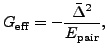$$G_{\text{eff}} = -\frac{\bar{\Delta}^2}{E_{\text{pair}}},$$ (47)

is determined from the HFB pairing energy,

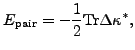$$E_{\text{pair}} = -\frac{1}{2}{\rm Tr}\Delta \kappa^* ,$$ (48)

and the average pairing gap ¹,

$$\bar{\Delta} = \frac{{\rm Tr'}\Delta \rho}{{\rm Tr}\rho} \, .$$ (49)

Expression (46) pertains to a system of particles occupying single-particle levels with fixed (non-self-consistent) energies and interacting with a seniority pairing interaction. In our method, this expression is used to probe the density of self-consistent energies that determine the curvature $\lambda_{2}$. All quantities defining $\lambda_{2}$ in Eq. (46) depend on the self-consistent solution and microscopic interaction, while the effective pairing strength $G_{\text{eff}}$ is only an auxiliary quantity. The quality of the prescription for calculating $\lambda_{2}$ can be tested against the exact VAPNP results (see Sec. 5).