Summary of HFB

We begin with the HFB approach. In what follows, we use the same notation as in Ref. [15]. The HFB formalism can be conveniently expressed in terms of the generalized density matrix, ${\cal R}$, defined as

$${\cal R} = \Bigg( \begin{array}{cc} \rho \quad & \kappa \\ -\kappa^{\ast } \quad & 1-\rho^{\ast } \end{array}\Bigg)\,\,\,\,,$$ (1)

where $\rho$ and $\kappa$ are the particle and pairing densities and ${\cal R}^2={\cal R}$. The energy variation results in the HFB equation

$$[{\cal W}, {\cal R}]=0\,\,\,,$$ (2)

which can be written as a non-linear eigenvalue problem:

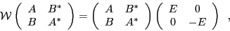$${\cal W}\left( \begin{array}{cc} A & B^\ast \\ B & A^\ast \e... ...t( \begin{array}{cc} E & 0 \\ 0 & -E \end{array}\right)\,\,\,,$$ (3)

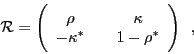
where

$${\cal W}= \left( \begin{array}{cc} h-\lambda & \Delta \\ -\Delta^{\ast} &-h^{\ast} + \lambda \end{array}\right) \,\,\, ,$$ (4)

$E$ is a diagonal matrix of quasiparticle energies $E_\mu$, $\lambda$ is the chemical potential, and matrices $h$ and $\Delta$ are the particle-hole and pairing mean-field potentials [1], respectively.

For the sake of comparison with the commonly used BCS formalism, it is quite useful to write the HFB equations in the canonical representation. The single-particle canonical wave function $\vert\mu\rangle$ can be expanded in the original single-particle (harmonic oscillator) basis $\vert n\rangle$ as

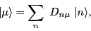$$\vert\mu\rangle = \sum_{n}~D_{n \mu} ~ \vert n\rangle,$$ (5)

where the unitary transformation $D$ is obtained by diagonalizing the density matrix $\rho$. In the canonical basis, the HFB wave function is given in a BCS-like form:

$$\breve{A}_{\mu \nu} = u_\mu \delta_{\mu \nu}\,\,\,,\,\,\, \breve{B}_{\mu \nu} = s_{\bar \mu}^\ast v_\mu \delta_{{\bar \mu} \nu},$$ (6)

$$u_\mu = u_{\bar \mu} = u_{\mu}^\ast\,\,\,,\,\,\,v_\mu = v_{\bar \mu} = v_{\mu}^\ast,$$ (7)

where the phase $s_{\mu}$, for the time-even quasiparticle vacuum considered here, is defined through the time-inversion of the single-particle states

$$\hat T \vert \mu \rangle = s_{\mu} \vert\bar \mu\rangle \,\,\,,\,\,\, s_{\bar \mu} = -s_{\mu}\,\,\,.$$ (8)

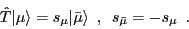
In Eq. (6) and in the following, the quantities in the canonical basis are denoted by symbols with breve accents [15].

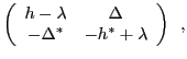
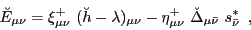
The HFB energy matrix $\breve{E}$ in the canonical basis is non-diagonal and is given by

$$\breve{E}_{\mu \nu} = \xi^+_{\mu \nu} ~(\breve{h}-\lambda)_... ...\nu}~\breve{\Delta}_{\mu \bar \nu}~s_{\bar \nu}^\ast \,\,\,,$$ (9)

where

$$\eta^{\pm}_{\mu \nu} = u_\mu v_\nu \pm u_\nu v_\mu \quad {\... ...} \quad \xi^{\pm}_{\mu \nu} = u_\mu u_\nu \mp v_\mu v_\nu \,.$$ (10)

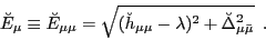
The diagonal matrix elements of the matrix $\breve{E}_{\mu \nu}$ can be written as [1,15]:

$$\breve{E}_{\mu} \equiv \breve{E}_{\mu \mu} = \sqrt{(\breve{h... ...u \mu} -\lambda)^2 + \breve{\Delta}_{\mu \bar \mu}^2}\,\,\,.$$ (11)

Even though the above equation resembles the BCS expression for quasiparticle energy, it involves $\breve{h}_{\mu \mu}$ and $\breve{\Delta}_{\mu \bar \mu}$, which are respectively obtained by transforming the HFB particle-hole and the pairing fields to the canonical basis via the transformation (5). It is only in the BCS approximation that these quantities can be associated with single-particle energies and the pairing gap.