Summary of ATDHFB

The ATDHFB approach is an approximation to the time-dependent HFB theory, wherein it is assumed that the collective velocity of the system is small compared to the average single-particle velocity of the nucleons. The generalized HFB density matrix is expanded around the quasi-stationary HFB solution ${\cal R}_0$ up to quadratic terms in the collective momentum:

$${ \cal R} = { \cal R}_0 + { \cal R}_1 + { \cal R}_2\,,$$ (12)

with ${\cal R}_1$ being time-odd and ${\cal R}_0$ and ${\cal R}_2$ time-even densities. The corresponding expansion for the HFB Hamiltonian reads

$${ \cal W} = { \cal W}_0 + { \cal W}_1 + { \cal W}_2.$$ (13)

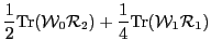
Employing the density expansion (12), the HFB energy can be separated into the collective kinetic and the potential parts. In terms of the density expansion (12), the kinetic energy is given by

$${\cal K} = \frac{1}{2} {\rm Tr} ( {\cal W}_0 { \cal R}_2 ) + \frac{1}{4}{\rm Tr} ( {\cal W}_1 { \cal R}_1 )$$

$$= \frac {i} {4} {\rm Tr} \left( {\dot {\cal R}_0} [{ \cal R}_0, { \... ...c {1} {2} \left( [ {\cal R}_2, { \cal R}_0] [{ \cal W}_0, { \cal R}_0] \right).$$ (14)

In the usual ATDHFB treatment, the second term involving ${\cal R}_2$ is neglected, and the kinetic energy can be written in the familiar form:

$${\cal K} = \frac {1} {2} {\dot q}^2 {\cal M} \,,$$ (15)

where the collective mass is given by

$${\cal M} = \frac {i} {2 {\dot q}^2} {\rm Tr} \biggr({\dot {\cal R}_0} [{\cal R}_0, {\cal R}_1] \biggr)$$ (16)

$$= \frac {i} {2 {\dot q}} {\rm Tr} \biggr( \frac {\partial {\cal R}_0} {\partial q} [{\cal R}_0, {\cal R}_1] \biggr).$$ (17)

The trace in the above expression can easily be evaluated in the quasiparticle basis. To this end, one can utilize the ATDHFB equation [3,4,5,6]

$$i {\dot {\cal R}_0} = [{\cal W}_0, {\cal R}_1 ] + [ {\cal W}_1, {\cal R}_0]\,.$$ (18)

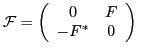
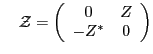
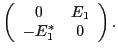
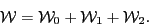
In the quasiparticle basis, the matrices ${\cal R}_0, {\cal W}_0, {\cal W}_1, {\cal R}_1$, and ${\dot {\cal R}_0}$ are represented by the matrices ${\cal G}, {\cal E}_0, {\cal E}_1, {\cal Z}$, and ${\cal F}$, respectively:

$${\cal R}_0 = {\cal A} {\cal G} {\cal A}^\dagger \,,$$ (19)

$${\cal W}_0 = {\cal A} {\cal E}_0 {\cal A}^\dagger \,,$$ (20)

$${\cal W}_1 = {\cal A} {\cal E}_1 {\cal A}^\dagger \,,$$ (21)

$${\cal R}_1 = {\cal A} {\cal Z} {\cal A}^\dagger \,,$$ (22)

$${\dot {\cal R}_0} = {\cal A} {\cal F} {\cal A}^\dagger \,,$$ (23)

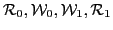
where

$${\cal A}= \left( \begin{array}{cc} A & B^\ast \\ B & A^\ast \end{array}\right)$$ (24)

is the matrix of the Bogolyubov transformation, and

$${\cal G} = \left( \begin{array}{cc} 0 & 0 \\ 0 & 1 \end{arr... ...\left( \begin{array}{cc} E & 0 \\ 0 & -E \end{array}\right) .$$ (25)

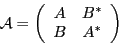
ATDHFB equation (18) can now be written in the quasiparticle basis as

$$i {\cal F} = [{\cal E}_0, {\cal Z} ] + [{\cal E}_1 \,, {\cal G}] \,.$$ (26)

This $2 \times 2$ matrix equation is, in fact, equivalent [6] to the following equation,

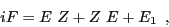$$i F = E~Z + Z~E + E_1\,\,\,,$$ (27)

where the antisymmetric matrices $F$, $Z$, and $E_1$ are related to ${\cal F}$, ${\cal Z}$, and ${\cal E}_1$:

$${\cal F} = \left( \begin{array}{cc} 0 & F \\ -F^\ast & 0 \end{array}\right) \quad , \quad {\cal Z} = \left( \begin{array}{cc} 0 & Z \\ -Z^\ast & 0 \end{array}\right)$$ (28)

$${}[{\cal E}_1 \,, {\cal G}] = \left( \begin{array}{cc} 0 & E_1 \\ -E_1^\ast & 0 \end{array}\right) .$$ (29)

In the case of several collective coordinates $\{q_i\}$, the ATDHFB equation (18) must be solved for each coordinate,

$$i {\dot q}_i\frac {\partial {\cal R}_0} {\partial q_i} = [{\cal W}_0, {\cal R}_1^i ] + [ {\cal W}_1^i, {\cal R}_0]\, ,$$ (30)

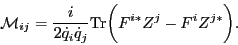
and the collective mass tensor becomes:

$${\cal M}_{ij} = \frac {i} {2\dot q_j} {\rm Tr} \biggr( \frac... ...\cal R}_0} {\partial q_i} [{\cal R}_0, {\cal R}_1^j] \biggr).$$ (31)

Then, in terms of the corresponding matrices $F^i$ and $Z^j$, the collective mass tensor is given by

$${\cal M}_{ij} = \frac {i} {2{\dot q_i} {\dot q_j}} {\rm Tr} \biggr( F^{i\ast} Z^j - F^i Z^{j\ast} \biggr).$$ (32)

The expression (32) for the mass tensor contains the matrix $Z^i$, which is associated with time-odd density matrix ${\cal R}_1^i$ and can, in principle, be obtained by solving the HFB equations with time-odd fields. The time-odd fields have been incorporated in mass-tensor calculations only in a limited number of cases. For instance, in Ref. [12], time-odd fields have been included in the HF study with a constraint of cylindrical symmetry. The time-odd fields have also been incorporated in the HFB study in an approximate iterative scheme with the collective path based on the Woods-Saxon potential [6].