Next: Central pseudopotential depending on Up: Cartesian representation of the Previous: Zero-order functional
At NLO, one obtains the EDF corresponding to the ![]() term of the
regularized pseudopotential (43) by applying on
all possible bilinear densities the relative-momentum operator:
term of the
regularized pseudopotential (43) by applying on
all possible bilinear densities the relative-momentum operator:
| (77) |
By taking the local limit of
functionals (79) and (80), we again recover the
quasilocal Cartesian EDF, which reads
 |
|||
| (80) |
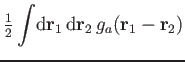
Finally, one obtains the EDF corresponding to the ![]() term of the
regularized pseudopotential (44) using the relative-momentum operator:
term of the
regularized pseudopotential (44) using the relative-momentum operator:
| (81) |
 |
|||
![$\textstyle +
{\textstyle{\frac{1}{4}}}(1-z_2)
\left[ \mathbf s_1\cdot\mathbf T_...
...frac{1}{4}}}\,\mathbf s_1\cdot\Delta\mathbf s_1-\mathbf J_1^2 \right]
\biggr\}.$](img342.png) |
(84) |
The second-order Cartesian EDF (79-80)
and (83-84) is exactly equivalent to that in the
spherical-tensor representation. The corresponding relations of
conversions between the parameters of the second-order regularized
pseudopotential (3) and those of its Cartesian
form (38) read
![$\displaystyle \biggl\{
A_1^{\rho_0}
\Bigl[
\left[{\textstyle{\frac{1}{2}}}\,\De...
...rho_0(\mathbf r_2)
+\mathbf j_0(\mathbf r_1)\cdot\mathbf j_0(\mathbf r_2)\Bigr]$](img297.png)
![$\displaystyle + A_1^{\rho_1}
\Bigl[
\left[{\textstyle{\frac{1}{2}}}\,\Delta\rho...
...rho_1(\mathbf r_2)
+\mathbf j_1(\mathbf r_1)\cdot\mathbf j_1(\mathbf r_2)\Bigr]$](img298.png)
![$\displaystyle + A_1^{\mathbf s_0}
\Bigl[
\left[{\textstyle{\frac{1}{2}}}\,\Delt...
...f s_0(\mathbf r_1)-\mathbf T_0(\mathbf r_1)\right]\cdot\mathbf s_0(\mathbf r_2)$](img299.png)
![$\displaystyle ~~~~~~~~
-{\textstyle{\frac{1}{4}}}\,\boldsymbol\nabla \otimes\ma...
... s_0(\mathbf r_2)
+\mathsf J_0(\mathbf r_1)\cdot\mathsf J_0(\mathbf r_2)
\Bigr]$](img300.png)
![$\displaystyle + A_1^{\mathbf s_1}
\Bigl[
\left[{\textstyle{\frac{1}{2}}}\,\Delt...
...f s_1(\mathbf r_1)-\mathbf T_1(\mathbf r_1)\right]\cdot\mathbf s_1(\mathbf r_2)$](img301.png)
![$\displaystyle ~~~~~~~~
-{\textstyle{\frac{1}{4}}}\,\boldsymbol\nabla \otimes\ma...
...hbf r_2)
+\mathsf J_1(\mathbf r_1)\cdot\mathsf J_1(\mathbf r_2)
\Bigr] \biggr\}$](img302.png)
![$\displaystyle \left.~~~~~~ -{\textstyle{\frac{1}{2}}}\boldsymbol\nabla \otimes\...
...thbf r_2,\mathbf r_1)\cdot\mathsf J_1(\mathbf r_1,\mathbf r_2)
\right]\biggr\}.$](img312.png)
![$\displaystyle \biggl\{
A_2^{\rho_0}
\left[ \rho_0(\mathbf r_1)\tau_0(\mathbf r_...
...o_0(\mathbf r_2)
-\mathbf j_0(\mathbf r_1)\cdot\mathbf j_0(\mathbf r_2)
\right]$](img327.png)
![$\displaystyle + A_2^{\mathbf s_1}
\left[ \mathbf s_1(\mathbf r_1)\cdot\mathbf T...
...bf r_2)
-\mathsf J_1(\mathbf r_1)\cdot\mathsf J_1(\mathbf r_2) \right]
\biggr\}$](img330.png)
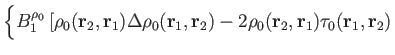
![$\displaystyle \biggl\{
B_2^{\rho_0}
\left[{\textstyle{\frac{1}{4}}}
\boldsymbol...
...bf r_2)
-\rho_0(\mathbf r_2,\mathbf r_1)\tau_0(\mathbf r_1,\mathbf r_2) \right]$](img332.png)
![$\displaystyle \left.~~~~~~ - \mathbf s_1(\mathbf r_2,\mathbf r_1)\cdot \mathbf T_1(\mathbf r_1,\mathbf r_2)
\right]
\biggr\},$](img337.png)