Cartesian representation of the central pseudopotential

In this section, we present derivation in the Cartesian representation of the nonlocal EDF that stems from the central ($\tilde{S}$=0) component of the regularized pseudopotential. This derivation is useful, because it establishes a clear connection of results presented in Sec. 2 with the Skyrme functional, which, in fact, constitutes the local limit of the nonlocal EDF. We used the explicit expressions for the Cartesian NLO functional, derived from the central finite-range pseudopotential, to benchmark their spherical counterparts. We checked explicitly that the two representations are equivalent when the relations between Cartesian and spherical local densities [9] and parameters of the interactions [11] were applied.

Following Refs. [3,17,26], we define the Cartesian form of the (non-antisymmetrized) central pseudopotential (2)-(3) in two equivalent representations as

$$\mathcal{V}_C = \sum_{nj} \left(W^{(n)}_j \hat{1}_\sigma\hat{1}_\tau+B^{(n)}_j \h... ...^{(n)}_j \hat{1}_\sigma\hat{P}^\tau-M^{(n)}_j \hat{P}^\sigma\hat{P}^\tau\right)$$

$$~~~~~~~~~~~~\times \hat{O}^{(n)}_j(\bm{k}',\bm{k})\delta(\bm{r}'_1-\bm{r}_1)\delta(\bm{r}'_2-\bm{r}_2) g_a(\bm{r}_1-\bm{r}_2)$$ (36)

and

$$\mathcal{V}_C = \sum_{nj} t^{(n)}_j \left( \hat{1}_\sigma\hat{1}_\tau+x^{(n)}_j \... ...^{(n)}_j \hat{1}_\sigma\hat{P}^\tau-z^{(n)}_j \hat{P}^\sigma\hat{P}^\tau\right)$$

$$~~~~~~~~\times \hat{O}^{(n)}_j(\bm{k}',\bm{k})\delta(\bm{r}'_1-\bm{r}_1)\delta(\bm{r}'_2-\bm{r}_2) g_a(\bm{r}_1-\bm{r}_2) ,$$ (37)

which contain the standard identity ( $\hat{1}_{\sigma,\tau}$) and exchange ( $\hat{P}^{\sigma,\tau}$) operators in spin and isospin spaces. In these expressions, indexes $n$ denote the orders of differential operators $\hat{O}^{(n)}_j(\bm{k}',\bm{k})$ and indexes $j$ number different operators of the same order. The first form, Eq. (37), generalizes the Gogny interaction by adding terms of higher orders $n>0$, whereas the second form, Eq. (38), generalizes the Skyrme interaction by adding two additional exchange terms. Obviously, the two forms are simply related one to another by the following relations between their strength parameters: $W^{(n)}_j=t^{(n)}_j$, $B^{(n)}_j=t^{(n)}_j x^{(n)}_j$, $H^{(n)}_j=t^{(n)}_j y^{(n)}_j$, and $M^{(n)}_j=t^{(n)}_j z^{(n)}_j$.

Differential operators $\hat{O}^{(n)}_j(\bm{k}',\bm{k})$ are scalar polynomial functions of two vectors, so owing to the GCH theorem [24], they must be polynomials of three elementary scalars: $\bm{k}^2$, $\bm{k}'^2$, and $\bm{k}'\cdot\bm{k}$. Hermiticity of the operators $\hat{O}^{(n)}_j(\bm{k}',\bm{k})$ can be enforced by using expressions symmetric with respect to exchanging $\bm{k}'^*$ and $\bm{k}$; therefore, it is convenient to build them from the following three scalars,

$$\hat{T}_1 = {\textstyle{\frac{1}{2}}}(\bm{k}'^*{}^2+ \bm{k}^2) ,$$ (38)

$$\hat{T}_2 = \bm{k}'^* \cdot\bm{k} ,$$ (39)

$$\hat{T}_3 = {\textstyle{\frac{1}{2}}}(\bm{k}'^*{}^2- \bm{k}^2) ,$$ (40)

with the condition that only even powers of $\hat{T}_3$ can appear. In terms of $\hat{T}_1$, $\hat{T}_2$, and $\hat{T}_3$, we now can define the following differential operators:

$$\hat{O}^{(0)}_1(\bm{k}',\bm{k}) = \hat{1} ,$$ (41)

$$\hat{O}^{(2)}_1(\bm{k}',\bm{k}) = \hat{T}_1 ,$$ (42)

$$\hat{O}^{(2)}_2(\bm{k}',\bm{k}) = \hat{T}_2 ,$$ (43)

$$\hat{O}^{(4)}_1(\bm{k}',\bm{k}) = \hat{T}_1^2+ \hat{T}_2^2 ,$$ (44)

$$\hat{O}^{(4)}_2(\bm{k}',\bm{k}) = 2\hat{T}_1 \hat{T}_2 ,$$ (45)

$$\hat{O}^{(4)}_3(\bm{k}',\bm{k}) = \hat{T}_1^2- \hat{T}_2^2 ,$$ (46)

$$\hat{O}^{(4)}_4(\bm{k}',\bm{k}) = \hat{T}_3^2 ,$$ (47)

$$\hat{O}^{(6)}_1(\bm{k}',\bm{k}) = \hat{T}_1^3+3\hat{T}_1 \hat{T}_2^2 ,$$ (48)

$$\hat{O}^{(6)}_2(\bm{k}',\bm{k}) = \hat{T}_2^3+3\hat{T}_1^2\hat{T}_2 ,$$ (49)

$$\hat{O}^{(6)}_3(\bm{k}',\bm{k}) = \hat{T}_1^3- \hat{T}_1 \hat{T}_2^2 ,$$ (50)

$$\hat{O}^{(6)}_4(\bm{k}',\bm{k}) = \hat{T}_2^3- \hat{T}_1^2\hat{T}_2 ,$$ (51)

$$\hat{O}^{(6)}_5(\bm{k}',\bm{k}) = \hat{T}_3^2\hat{T}_1 ,$$ (52)

$$\hat{O}^{(6)}_6(\bm{k}',\bm{k}) = \hat{T}_3^2\hat{T}_2 .$$ (53)

Because for every operator $\hat{O}^{(n)}_j(\bm{k}',\bm{k})$ there appear in Eqs. (37) and (38) four different spin-isospin terms, we recover here the numbers of central terms shown in Table 1.

Of course, at any given order, the choice of polynomials of $\hat{T}_1$, $\hat{T}_2$, and $\hat{T}_3$ is quite arbitrary - with only requirement that these polynomials be linearly independent. Definitions (42)-(54) were chosen so as to naturally link them to the standard Skyrme interaction, for which we have

$$t_0 = t^{(0)}_1, \quad x_0 = x^{(0)}_1 ,$$ (54)

$$t_1 = t^{(2)}_1, \quad x_1 = x^{(2)}_1 ,$$ (55)

$$t_2 = t^{(2)}_2, \quad x_2 = x^{(2)}_2 ,$$ (56)

and to encompass definitions of fourth-order parameters $t^{(4)}_1$, $t^{(4)}_2$, $x^{(4)}_1$, and $x^{(4)}_2$ introduced in Ref. [26]. For a lighter notation used below, we also define the analogous parameters:

$$y_0 = y^{(0)}_1, \quad z_0 = z^{(0)}_1 ,$$ (57)

$$y_1 = y^{(2)}_1, \quad z_1 = z^{(2)}_1 ,$$ (58)

$$y_2 = y^{(2)}_2, \quad z_2 = z^{(2)}_2 .$$ (59)

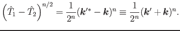
At higher orders, we picked the $j=1$ and 2 terms so as to have at any order $n>0$,

$$\hspace*{-1cm} \hat{O}^{(n)}_1(\bm{k}',\bm{k}) - \hat{O}^{(n)}_2(\bm{k}',\bm{k}) = \left(\hat{T}_1-\hat{T}_2\right)^{n/2} = \frac{1}{2^n}(\bm{k}'^*-\bm{k})^n \equiv \frac{1}{2^n}(\bm{k}'+\bm{k})^n .$$ (60)

These particular polynomials of relative momenta are special [3], because, as it turns out, the sum of relative-momentum operators $\bm{k}'+\bm{k}$ commutes with the locality deltas, see Sec. 5.

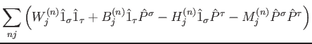
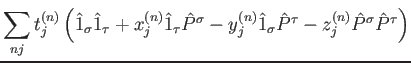
In the following we give separate expressions for the functional derived from three lowest-order terms (42)-(44) of the pseudopotential, denoting them by $\langle V_i \rangle$ for $i=0$, 1, and 2. We also separate the local and non local terms, denoting them, respectively, by $\langle V_i^L\rangle$ and $\langle V_i^{N}\rangle$. To have more compact expressions, we also introduced the following combinations of parameters of the regularized interaction (55)-(60):

$$A^{\rho_0}_i = \phantom{-}{\textstyle{\frac{1}{2}}}\, t_i\left(1+{\textstyle{\fr... ...2}}}\,x_i-{\textstyle{\frac{1}{2}}}\,y_i-{\textstyle{\frac{1}{4}}}\,z_i\right),$$ (61)

$$A^{\rho_1}_i = - {\textstyle{\frac{1}{2}}}\, t_i\left({\textstyle{\frac{1}{2}}}\,y_i+{\textstyle{\frac{1}{4}}}\,z_i\right) ,$$ (62)

$$A^{\bm{s}_0}_i = \phantom{-}{\textstyle{\frac{1}{2}}}\, t_i\left({\textstyle{\frac{1}{2}}}\,x_i-{\textstyle{\frac{1}{4}}}\,z_i\right) ,$$ (63)

$$A^{\bm{s}_1}_i = - {\textstyle{\frac{1}{8}}}\, t_iz_i ,$$ (64)

$$B^{\rho_0}_i = -{\textstyle{\frac{1}{2}}}\, t_i\left({\textstyle{\frac{1}{4}}}+{\textstyle{\frac{1}{2}}}\,x_i-{\textstyle{\frac{1}{2}}}\,y_i-z_i\right) ,$$ (65)

$$B^{\rho_1}_i = -{\textstyle{\frac{1}{2}}}\, t_i\left({\textstyle{\frac{1}{4}}}+{\textstyle{\frac{1}{2}}}\,x_i\right) ,$$ (66)

$$B^{\bm{s}_0}_i = -{\textstyle{\frac{1}{2}}}\, t_i\left({\textstyle{\frac{1}{4}}}-{\textstyle{\frac{1}{2}}}\,y_i\right) ,$$ (67)

$$B^{\bm{s}_1}_i = -{\textstyle{\frac{1}{8}}}\, t_i.$$ (68)