Apart from the 4242 configuration discussed above, in 60Zn we
also calculated 6 other configurations, namely those that correspond
to exciting the 42 proton and neutron simultaneously to the
negative-parity orbitals ![]() and
and ![]() .
In principle, there are
16 such excitations possible, however, the lowest ones are obtained
by putting the neutron and the proton in the same orbitals.
This gives 4 configurations denoted by
41f+41f+,
41f-41f-,
41p+41p+, and
41p-41p-. In addition, we
also study 2 other configurations obtained by putting the neutron and
the proton into the [303]7/2 orbital with different signatures,
i.e., those denoted by
41f+41f- and
41f-41f+.
.
In principle, there are
16 such excitations possible, however, the lowest ones are obtained
by putting the neutron and the proton in the same orbitals.
This gives 4 configurations denoted by
41f+41f+,
41f-41f-,
41p+41p+, and
41p-41p-. In addition, we
also study 2 other configurations obtained by putting the neutron and
the proton into the [303]7/2 orbital with different signatures,
i.e., those denoted by
41f+41f- and
41f-41f+.
In Fig. 7(b) the energies of the seven configurations
selected above are shown with respect to a common rigid-rotor
reference energy of 0.025![]() I(I+1)MeV. Similarly,
Figs. 7(a) and (c) show the analogous configurations in
58Cu and 62Ga. Because orbitals
I(I+1)MeV. Similarly,
Figs. 7(a) and (c) show the analogous configurations in
58Cu and 62Ga. Because orbitals ![]() and
and ![]() are very
close in energy (cf. Fig. 1), they strongly interact and
mix, which very often precludes the convergence of the HF procedure,
see discussion in Ref. [36]. Apart from that, the bands of
Fig. 7 are shown up to the so-called termination points,
i.e., up to the point where the angular-momentum contents of the
involved orbitals does not allow for a further angular momentum build
up, see Ref. [37], without a significant rearrangement of
the nucleons.
are very
close in energy (cf. Fig. 1), they strongly interact and
mix, which very often precludes the convergence of the HF procedure,
see discussion in Ref. [36]. Apart from that, the bands of
Fig. 7 are shown up to the so-called termination points,
i.e., up to the point where the angular-momentum contents of the
involved orbitals does not allow for a further angular momentum build
up, see Ref. [37], without a significant rearrangement of
the nucleons.
By considering the available projections of the total angular momentum Iy for oblate shapes with the y axis as the symmetry axis, one can easily determine the values of the termination-point angular momenta It, see Table 2. The bands obtained in the HF calculations do not always terminate at the oblate axis and can usually be continued beyond It. However, at angular momenta It there always occur significant changes in the structure of bands. Below we discuss and present results only up to the termination points It.
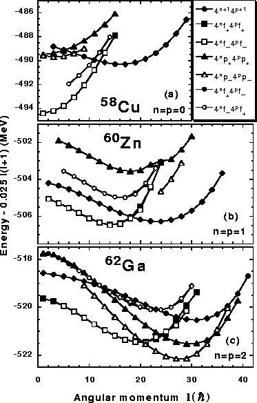 |
A conspicuous feature of the HF energies presented in
Fig. 7 is the significant energy separation between the
n-p paired configurations
4nf+4pf+ and
4nf-4pf- on one
side, and the broken-pair configurations
4nf+4pf- and
4nf-4pf+ on the other side. The former and latter
configurations have opposite total signatures, i.e., in the even-even
nucleus 60Zn, configurations
41f+41f+ and
41f-41f-(
41f+41f- and
41f-41f+) correspond to r=+1 (r=-1),
while in the odd-odd nuclei 58Cu and 62Ga the analogous
configurations correspond to r=-1 (r=+1). Such a
signature-separation effect has been for the first time discussed for
the SD bands in 32S [38]. Here it is obtained in the
heavier SD region of the A![]() 60 nuclei, as a mutatis mutandis
identical effect occurring for all the orbitals promoted to the next
HO shell.
60 nuclei, as a mutatis mutandis
identical effect occurring for all the orbitals promoted to the next
HO shell.
| Configuration |
|
|
|
|||||||
| 4n+14p+1 | [2(p+1),2(n+1)] | 29 | 36 | 41 | ||||||
| 4nf+4pf+ | [1p,1n] | 15 | 24 | 31 | ||||||
| 4nf-4pf- | [1p,1n] | 13 | 22 | 29 | ||||||
| 4np+4pp+ | [2p,2n] | 23 | 32 | 39 | ||||||
| 4np-4pp- | [2p,2n] | 21 | 30 | 37 | ||||||
| 4nf+4pf- | [1p,1n] | 14 | 23 | 30 | ||||||
| 4nf-4pf+ | [1p,1n] | 14 | 23 | 30 | ||||||
In Ref. [38] the signature-separation effect was
interpreted as a result of the strong n-p attraction transmitted
through the time-odd mean fields. Such an attraction is typical for
any realistic effective interaction, and it has its origin in the
spin-spin components of the interaction. (The signature separation
vanishes when in the Skyrme energy functional [39] the
coupling constants corresponding to terms
![]()
![]()
![]() and
and
![]()
![]()
![]() are set equal to zero.) When
averaged within the mean-field approximation, the spin-spin
components lead naturally to the time-odd mean fields
[39]. Within the phenomenological mean fields, like those
given by the Woods-Saxon or Nilsson potentials [40], the
time-odd mean fields vanish, and therefore all the four configurations
are set equal to zero.) When
averaged within the mean-field approximation, the spin-spin
components lead naturally to the time-odd mean fields
[39]. Within the phenomenological mean fields, like those
given by the Woods-Saxon or Nilsson potentials [40], the
time-odd mean fields vanish, and therefore all the four configurations
![]() are nearly degenerate, i.e., the
signature-separation effect occurs only for self-consistent mean
fields generated from the spin-spin interactions.
are nearly degenerate, i.e., the
signature-separation effect occurs only for self-consistent mean
fields generated from the spin-spin interactions.
One should note that the four configurations
![]() have
purely independent-particle character (Slater-determinant wave
functions), i.e., no collective pair correlations are built into the
wave functions. Nevertheless, configurations
4nf+4pf+ and
4nf-4pf- contain one more T=0 n-p pair as compared to the
4nf+4pf- and
4nf-4pf+ configurations, and therefore are
sensitive to the n-p pairing component of the effective interaction
that is attractive. As a result, the paired configurations
4nf+4pf+ and
4nf-4pf- cross the magic configurations
4n+14p+1 at I=11, 18, and 27
have
purely independent-particle character (Slater-determinant wave
functions), i.e., no collective pair correlations are built into the
wave functions. Nevertheless, configurations
4nf+4pf+ and
4nf-4pf- contain one more T=0 n-p pair as compared to the
4nf+4pf- and
4nf-4pf+ configurations, and therefore are
sensitive to the n-p pairing component of the effective interaction
that is attractive. As a result, the paired configurations
4nf+4pf+ and
4nf-4pf- cross the magic configurations
4n+14p+1 at I=11, 18, and 27![]() in 58Cu, 60Zn,
and 62Ga, respectively.
in 58Cu, 60Zn,
and 62Ga, respectively.
The n-p pairing correlations should be, in principle, studied by using methods beyond the mean-field approximation, i.e., by taking into account the configuration-mixing effects for configurations that differ by the n-p pair occupations. The generator-coordinate method (GCM) [40] is the approach of choice for including such effects. It allows for a consistent improvement of wave functions, while staying in the framework of the variational approach. Therefore, the same interaction can be/should be used in the HF method and in the mixing of the HF configurations via the GCM method.
At present, the GCM approach in the rotating frame has not yet been
implemented, and in the present study we discuss the same physics
problem by introducing a model T=0 n-p pair-interaction Hamiltonian
in the form of
Hamiltonian (1) is meant to replace the usual
effective-interaction (Skyrme) Hamiltonian when studying the n-p
correlation aspects of the nuclear wave functions, and not to be
added on top of it. Therefore, the effective single-particle energies
![]() and the coupling constants
and the coupling constants
![]() =
=
![]() have to be
angular-momentum and configuration dependent, and Hamiltonian
(1) should be understood as a phenomenological interaction
operator between configurations that differ by the n-p pair
occupations.
have to be
angular-momentum and configuration dependent, and Hamiltonian
(1) should be understood as a phenomenological interaction
operator between configurations that differ by the n-p pair
occupations.
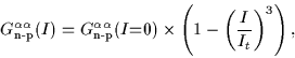
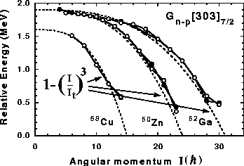
The diagonal pairing term can be transformed as
By subtracting the total HF energies of configurations in
Eq. (8), see Fig. 7, one thus obtains an
estimate of the n-p pairing diagonal matrix element
![]() .
Such relative energies (8) in
58Cu, 60Zn, and 62Ga are plotted in Fig. 8. One
can see that the effective matrix elements depend strongly on the
angular momentum, and decrease from
.
Such relative energies (8) in
58Cu, 60Zn, and 62Ga are plotted in Fig. 8. One
can see that the effective matrix elements depend strongly on the
angular momentum, and decrease from
![]() =0)
=0)![]() 1.6 (58Cu) or 1.9MeV
(60Zn and 62Ga), reaching zero at the termination angular
momentum It. This dependence can be very well parameterized by a
simple cubic expression,
1.6 (58Cu) or 1.9MeV
(60Zn and 62Ga), reaching zero at the termination angular
momentum It. This dependence can be very well parameterized by a
simple cubic expression,
 |
A large standard signature splitting of the other single-particle
orbitals, which have lower values of the K quantum numbers, does
not allow us to determine the other diagonal matrix elements
![]() directly from the HF results, as in
Eq. (8). Of course, such a determination of the
non-diagonal matrix elements is not possible either. However, we may
use the I-dependence of Eq. (9) to postulate a simple
separable approximation for the n-p pairing interaction matrix
directly from the HF results, as in
Eq. (8). Of course, such a determination of the
non-diagonal matrix elements is not possible either. However, we may
use the I-dependence of Eq. (9) to postulate a simple
separable approximation for the n-p pairing interaction matrix
![]() in the form
in the form
Within the separable approximation (10), the T=0 n-p
pairing interaction
![]() in Hamiltonian (1) takes
the simple form of
in Hamiltonian (1) takes
the simple form of
 |
 |
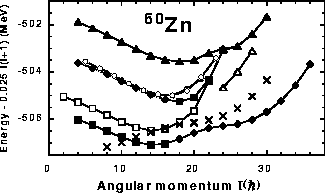
Before these become available, in the present study we perform the
simplest two-level mixing calculation, in which the two
configurations that cross in 60Zn, 4242 and
41f+41f+,
see Fig. 7(b), are allowed to interact through the T=0
n-p pairing interaction (11). With the diagonal matrix
elements of Hamiltonian (1) taken from the HF calculations,
and the interaction matrix element defined by the value of
![]() [303]7/2(I=0)=1.9MeV, also taken from the HF
calculations, we are left with one free parameter, i.e., with the
value of
[303]7/2(I=0)=1.9MeV, also taken from the HF
calculations, we are left with one free parameter, i.e., with the
value of
![]() [440]1/2(I=0).
[440]1/2(I=0).
By fixing this parameter at
![]() [440]1/2(I=0) = 0.65MeV, we
obtain at the crossing point of I=18
[440]1/2(I=0) = 0.65MeV, we
obtain at the crossing point of I=18![]() the effective
interaction strength of 0.79MeV. With the I-dependent matrix
elements given by Eqs. (9) and (10), we obtain the
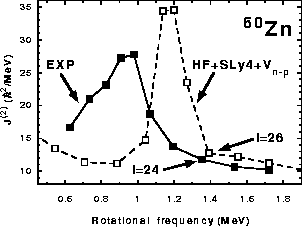
energies and dynamic moments of inertia shown in Figs. 9
and 10, respectively. It is clear that the mixing and
interaction of the 4242 and
41f+41f+ configurations
correctly reproduces the magnitude of the bump in the
the effective
interaction strength of 0.79MeV. With the I-dependent matrix
elements given by Eqs. (9) and (10), we obtain the
energies and dynamic moments of inertia shown in Figs. 9
and 10, respectively. It is clear that the mixing and
interaction of the 4242 and
41f+41f+ configurations
correctly reproduces the magnitude of the bump in the
![]() of
60Zn.
of
60Zn.
The position of the crossing point is obtained at frequency or spin
that are too large by 0.2MeV or 4![]() ,
respectively, as
compared to experiment. As seen in Fig. 7(b),
this position is dictated by the diagonal matrix element
,
respectively, as
compared to experiment. As seen in Fig. 7(b),
this position is dictated by the diagonal matrix element
![]() [303]7/2 that shifts down configuration
41f+41f+ with
respect to the broken-pair degenerate configurations
41f+41f-and
41f-41f+. As discussed above, such a shift is a direct
consequence of the time-odd mean fields resulting from the Skyrme
energy density. In the present work we have used the time-odd terms
as directly given by the SLy4 Skyrme functional, see
Ref.[39], i.e., those that result from fitting the
time-even, and not time-odd properties of nuclei. It is clear that a
modification of these time-odd terms, that is permitted in the local
density approximation, may move the crossing frequency from its
current position in Fig. 10. In fact, it is obvious that
by decreasing this intensity one may easily decrease the crossing
frequency. We do not attempt such a fit here, because the problem of
finding good physical values of the time-odd coupling constants is
much more general, and it would not make too much sense to make such
an adjustment based solely on the specific effect discussed in the
present study. We only note in passing that an analogous readjustment
of the isovector time-odd coupling constants[41] has led to
values that are quite different from those resulting directly from
the Skyrme functional.
[303]7/2 that shifts down configuration
41f+41f+ with
respect to the broken-pair degenerate configurations
41f+41f-and
41f-41f+. As discussed above, such a shift is a direct
consequence of the time-odd mean fields resulting from the Skyrme
energy density. In the present work we have used the time-odd terms
as directly given by the SLy4 Skyrme functional, see
Ref.[39], i.e., those that result from fitting the
time-even, and not time-odd properties of nuclei. It is clear that a
modification of these time-odd terms, that is permitted in the local
density approximation, may move the crossing frequency from its
current position in Fig. 10. In fact, it is obvious that
by decreasing this intensity one may easily decrease the crossing
frequency. We do not attempt such a fit here, because the problem of
finding good physical values of the time-odd coupling constants is
much more general, and it would not make too much sense to make such
an adjustment based solely on the specific effect discussed in the
present study. We only note in passing that an analogous readjustment
of the isovector time-odd coupling constants[41] has led to
values that are quite different from those resulting directly from
the Skyrme functional.