The asymptotic properties of the two components of the HFB
quasiparticle wave functions, and their dependence on ![]() and
and
![]() , were discussed in Refs. [17,5,18]. Here we
complement this discussion by further elements, which pertain mainly
to weakly bound systems where the Fermi energy
, were discussed in Refs. [17,5,18]. Here we
complement this discussion by further elements, which pertain mainly
to weakly bound systems where the Fermi energy ![]() is very
small.
is very
small.
Assuming that ![]() =
=
![]() , which anyhow is always
fulfilled in the asymptotic region, and neglecting for simplicity
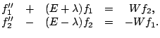
this trivial mass factor altogether, Eqs. (34) have for
large
, which anyhow is always
fulfilled in the asymptotic region, and neglecting for simplicity
this trivial mass factor altogether, Eqs. (34) have for
large ![]() the following form
the following form
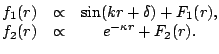
In order to discuss this question, we note that the coupling terms can be considered as inhomogeneities of the linear equations (35), and therefore, asymptotic solutions have the form
We arrive here at the conclusion that the asymptotic form of ![]() may involve two terms and a more detailed analysis is needed before
concluding which one dominates. To this end, we note that the coupling
potential
may involve two terms and a more detailed analysis is needed before
concluding which one dominates. To this end, we note that the coupling
potential ![]() depends on the sum of products of lower and upper
components, and therefore has a general form of
depends on the sum of products of lower and upper
components, and therefore has a general form of
| (36) |
In order to illustrate the above discussion, we have performed the
HFB calculations in ![]() Sn, where
Sn, where ![]() =
=![]() 0.345MeV and
the lowest
0.345MeV and
the lowest ![]() =0 quasiparticle state of
=0 quasiparticle state of ![]() =0.429MeV (for
=0.429MeV (for
![]() =30fm) leads to a very diffused coupling
potential with small decay constant
=30fm) leads to a very diffused coupling
potential with small decay constant ![]() . Quasiparticle wave
functions corresponding to the four lowest
. Quasiparticle wave
functions corresponding to the four lowest ![]() =0 quasiparticle
states are shown in Fig. 1. One can see that the asymptotic
forms of the second components
=0 quasiparticle
states are shown in Fig. 1. One can see that the asymptotic
forms of the second components ![]() of the two lowest
quasiparticle states are not affected by the second term
of the two lowest
quasiparticle states are not affected by the second term ![]() , at
least up to 30fm. Only the third and fourth states switch at large
distances to the oscillating asymptotic forms with a smaller decay
constant. This happens at rather large distances where the densities
are anyhow very small. Hence the change in the asymptotic properties
does not affect any important nuclear observables.
, at
least up to 30fm. Only the third and fourth states switch at large
distances to the oscillating asymptotic forms with a smaller decay
constant. This happens at rather large distances where the densities
are anyhow very small. Hence the change in the asymptotic properties
does not affect any important nuclear observables.
In all cases that we have studied, the practical importance of the
second term ![]() is negligible. However, its presence precludes
simple analytic continuation of the wave functions in the asymptotic
region. We would like to stress that the asymptotic forms discussed
in this section are numerically stable, and that they are unrelated
to the numerical instabilities discussed in Sec. 5.3 below.
is negligible. However, its presence precludes
simple analytic continuation of the wave functions in the asymptotic
region. We would like to stress that the asymptotic forms discussed
in this section are numerically stable, and that they are unrelated
to the numerical instabilities discussed in Sec. 5.3 below.
![$ \begin{matrix}
\includegraphics*[scale=0.45,clip,bb=62 53 490 340]{wf1.ps} &
\...
... &
\includegraphics*[scale=0.45,clip,bb=62 53 490 340]{wf4.ps} \\
\end{matrix}$](img147.png)