Energy density at N$\bm {{}^3}$LO with conserved spherical, space-inversion, and time-reversal symmetries

In this section, we apply the results obtained above to the simplest case of spherical even-even nuclei [28], where one can assume that the spherical symmetry, along with the space inversion and time reversal, are simultaneously conserved symmetries. In this case, all primary densities $\rho_{nLvJ}$ (23), which we listed in Tables 3 and 4, must have the form [39]:

$$\rho_{nLvJ}(\vec {r})=R_{JJ}(\vec {r})\rho_{nLvJ}(\vert\vec {r}\vert),$$ (44)

where

$$R_{JJ}(\vec {r})=[r[r\ldots,[rr]_2,\ldots,]_{J-2}]_J$$ (45)

is the $J$th-order, rank-$J$ stretched coupled tensor built from the position vector $\vec {r}$ in exactly the same way as the derivative operators $D_{nL}$ of Table 1 are built from the derivative $\vec {\nabla}$ in the spherical representation (9), and $\rho_{nLvJ}(\vert\vec {r}\vert)$ is a scalar function depending only on the length $\vert\vec {r}\vert$ of the position vector $\vec {r}$.

Indeed, due to the generalized Cayley-Hamilton (GCH) theorem, a rank-$J$ tensor function of a rank-$k$ tensor must be a linear combination of all independent rank-$J$ tensors built from that rank-$k$ tensor, with scalar coefficients. In the GCH theorem, tensors that differ by scalar factors are not independent. In our case, only one independent rank-$J$ function $R_{JJ}(\vec {r})$ can be built from the rank-1 tensor (position vector $\vec {r}$), which gives Eq. (44). The spherical symmetry assumed here is essential for this argument to work, because many more independent rank-$J$ tensors can be built when other ``material'' tensors (like, e.g., the quadrupole deformation tensor) are available.

The spherical form of $\rho_{nLvJ}(\vec {r})$ (44) requires that the following selection rule is obeyed:

$$P = (-1)^J,$$ (46)

where $P=(-1)^n$ is the space-inversion parity defined in Eq. (26). For the time-even densities ($T=1$), selection rule (46) does not impose any new restriction on local densities built from $\rho\left(\vec {r},\vec {r}'\right)$ ($v=0$), see Table 3. On the other hand, for local densities built from $\vec {s}\left(\vec {r},\vec {r}'\right)$ ($v=1$), see Table 4, only the densities with $L=J$ are allowed.

In Tables 3 and 4, all densities allowed by the conserved spherical, space-inversion, and time-reversal symmetries are marked with bullets ($\bullet$). One can see that they correspond to quantum numbers $LvJ$ being equal to 000 or 202 [for densities built from $\rho\left(\vec {r},\vec {r}'\right)$] and 111 or 313 [for densities built from $\vec {s}\left(\vec {r},\vec {r}'\right)$]. Then, it is easy to select all allowed terms in the energy density--in Tables 7-18 and 22 these are also marked with bullets ($\bullet$). Numbers of such terms are listed in Table 20 together with those obtained by imposing, in addition, the Galilean or gauge invariance.

Table 20: Numbers of terms defined in Eq. (30) of different orders in the EDF up to N$^3$LO, evaluated for the conserved spherical, space-inversion, and time-reversal symmetries. The last two columns give numbers of terms when the Galilean or gauge invariance is assumed, respectively, see Sec. 3.2. To take into account both isospin channels, the numbers of terms should be multiplied by a factor of two.

order	Total	Galilean	Gauge
0	1	1	1
2	4	4	4
4	13	9	3
6	32	16	3
N$^3$LO	50	30	11

All results for the EDF restricted by the spherical, space-inversion, and time-reversal symmetries can now be extracted from the general results presented in Secs. 2 and 3 and Appendices B and C. However, in the remainder of this section we give an example of how these results can be translated into those based on the Cartesian representations of derivative operators (18)-(22). Indeed, in this representation, all non-zero densities can be defined as:

$$R_{0} = \rho ,$$ (47)

$$R_{2} = \vec {k}^2\rho ,$$ (48)

$$\stackrel{\leftrightarrow}{R}_{2ab} = \vec {k}_a\vec {k}_b\rho ,$$ (49)

$$R_{4} = \vec {k}^4\rho ,$$ (50)

$$\stackrel{\leftrightarrow}{R}_{4ab} = \vec {k}^2\vec {k}_a\vec {k}_b\rho ,$$ (51)

$$R_{6} = \vec {k}^6\rho ,$$ (52)

and

$$\vec {J}_{1a} = (\vec {k}\times\vec {s})_a ,$$ (53)

$$\vec {J}_{3a} = \vec {k}^2(\vec {k}\times\vec {s})_a ,$$ (54)

$$\stackrel{\leftrightarrow}{J}_{3abc} = \vec {k}_a\vec {k}_b(\vec {k}\times\vec {s})_c + \vec {k}_b\vec {k}_c(\vec {k}\times\vec {s})_a$$

$$+ \vec {k}_c\vec {k}_a(\vec {k}\times\vec {s})_b ,$$ (55)

$$\vec {J}_{5a} = \vec {k}^4(\vec {k}\times\vec {s})_a ,$$ (56)

where

$$\vec {k}^2 = \sum_a\vec {k}_a\vec {k}_a ,$$ (57)

and the Cartesian indices are defined as $a, b, c=x, y, z$. To lighten the notation, in these definitions we have omitted the arguments of local densities, $\vec {r}$, and limits of $\vec {r}'=\vec {r}$.

The six local densities (47)-(52) are the Cartesian analogues of densities marked in Table 3 with bullets ($\bullet$), and the four local densities (53)-(56) are analogues of those marked in Table 4. However, one should note that rank-2 densities $\stackrel{\leftrightarrow}{R}_{2ab}$ and $\stackrel{\leftrightarrow}{R}_{4ab}$ are not proportional to $\rho_{2202}$ and $\rho_{4202}$, respectively, and the rank-3 density $\stackrel{\leftrightarrow}{J}_{3abc}$ is not proportional to $\rho_{3313}$. This is so, because they are defined in terms of the derivative operators (18)-(22), where appropriate traces have not been subtracted out. Nevertheless, linear relations between densities (47)-(56) and their spherical-representation counterparts $\rho_{nLvJ}$ can easily be worked out and will not be presented here.

Note also that the scalar densities $R_{2}$ and $R_{4}$ can be expressed as the corresponding sums of the rank-2 densities $\stackrel{\leftrightarrow}{R}_{2ab}$ and $\stackrel{\leftrightarrow}{R}_{4ab}$, and the vector density $\vec {J}_{3a}$ as that of $\stackrel{\leftrightarrow}{J}_{3abc}$. However, based on the results obtained in the spherical representation, we know that they have to be treated separately to give separate terms in the energy density.

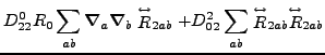
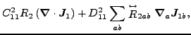
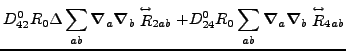
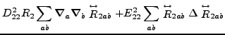
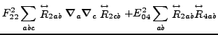
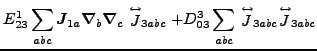
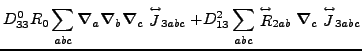
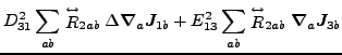
Again, based on the results obtained in the spherical representation, we can write the N$^3$LO energy density as a sum of contributions from zero, second, fourth, and sixth orders:

$${\cal H} = {\cal H}_0 + {\cal H}_2 + {\cal H}_4 + {\cal H}_6 ,$$ (58)

where

$${\cal H}_0 = C^0_{00} R_0R_0 ,$$ (59)

$${\cal H}_2 = C^0_{20} R_0\Delta R_0 + C^0_{02} R_0R_2$$

$$+ C^0_{11} R_0 \vec {\nabla}\cdot\vec {J}_1, + C^1_{01} \vec {J}_1^2,$$ (60)

Energy densities ${\cal H}_0$ and ${\cal H}_2$ correspond, of course, to the standard Skyrme functional [36,24] with $C^0_{00}=C^\rho$, $C^0_{20}=C^{\Delta\rho}$, $C^0_{02}=C^\tau$, $C^0_{11}=C^{\nabla{J}}$, and $C^1_{01}=C^{J1}$. At fourth and sixth orders, these energy densities read

$${\cal H}_4 = C^0_{40} R_0\Delta^2 R_0 + C^0_{22} R_0\Delta R_2$$

$$+ C^0_{04} R_0R_4 + C^2_{02} R_2R_2$$

$$+ D^0_{22} R_0\sum_{ab}\vec {\nabla}_a\vec {\nabla}_b \stackrel{\le... ...um_{ab} \stackrel{\leftrightarrow}{R}_{2ab} \stackrel{\leftrightarrow}{R}_{2ab}$$

$$+ C^1_{21} \vec {J}_1\cdot\Delta \vec {J}_1 + C^1_{03} \vec {J}_1\cdot\vec {J}_3$$

$$+ D^1_{21} \vec {J}_1\cdot\vec {\nabla}\left(\vec {\nabla}\cdot\vec {J}_1\right)$$

$$+ C^0_{31} R_0\Delta\left(\vec {\nabla}\cdot\vec {J}_1\right) + C^0_{13} R_0\left(\vec {\nabla}\cdot\vec {J}_3\right)$$

$$+ C^2_{11} R_2\left(\vec {\nabla}\cdot\vec {J}_1\right) + D^2_{11} \sum_{ab} \stackrel{\leftrightarrow}{R}_{2ab} \vec {\nabla}_a \vec {J}_{1b} ,$$ (61)

$${\cal H}_6 = C^0_{60} R_0\Delta^3 R_0 + C^0_{42} R_0\Delta^2 R_2$$

$$+ C^0_{24} R_0\Delta R_4 + C^0_{06} R_0R_6$$

$$+ C^2_{22} R_2\Delta R_2 + C^2_{04} R_2R_4$$

$$+ D^0_{42} R_0\Delta\sum_{ab}\vec {\nabla}_a\vec {\nabla}_b \stackr... ... R_0\sum_{ab}\vec {\nabla}_a\vec {\nabla}_b \stackrel{\leftrightarrow}{R}_{4ab}$$

$$+ D^2_{22} R_2\sum_{ab}\vec {\nabla}_a\vec {\nabla}_b \stackrel{\le... ...} \stackrel{\leftrightarrow}{R}_{2ab}\Delta \stackrel{\leftrightarrow}{R}_{2ab}$$

$$+ F^2_{22} \sum_{abc}\stackrel{\leftrightarrow}{R}_{2ab}\vec {\nabl... ...um_{ab} \stackrel{\leftrightarrow}{R}_{2ab} \stackrel{\leftrightarrow}{R}_{4ab}$$

$$+ C^1_{41} \vec {J}_1\cdot\Delta^2 \vec {J}_1 + C^1_{23} \vec {J}_1\cdot\Delta\vec {J}_3$$

$$+ C^1_{05} \vec {J}_1\cdot \vec {J}_5 + C^3_{03} \vec {J}_3\cdot \vec {J}_3$$

$$+ D^1_{41} \vec {J}_1\cdot\Delta\vec {\nabla}\left(\vec {\nabla}\cd... ... D^1_{23} \vec {J}_1\cdot\vec {\nabla}\left(\vec {\nabla}\cdot\vec {J}_3\right)$$

$$+ E^1_{23} \sum_{abc}\vec {J}_{1a}\vec {\nabla}_b\vec {\nabla}_c \s... ...{abc} \stackrel{\leftrightarrow}{J}_{3abc} \stackrel{\leftrightarrow}{J}_{3abc}$$

$$+ C^0_{51} R_0\Delta^2\left(\vec {\nabla}\cdot\vec {J}_1\right) + C^0_{33} R_0\Delta\left(\vec {\nabla}\cdot\vec {J}_3\right)$$

$$+ C^0_{15} R_0\left(\vec {\nabla}\cdot\vec {J}_5\right) + C^2_{31} R_2\Delta\left(\vec {\nabla}\cdot\vec {J}_1\right)$$

$$+ C^2_{13} R_2\left(\vec {\nabla}\cdot\vec {J}_3\right) + C^4_{11} R_4\left(\vec {\nabla}\cdot\vec {J}_1\right)$$

$$+ D^0_{33} R_0\sum_{abc}\vec {\nabla}_{a}\vec {\nabla}_b\vec {\nabl... ...el{\leftrightarrow}{R}_{2ab}\vec {\nabla}_c\stackrel{\leftrightarrow}{J}_{3abc}$$

$$+ D^2_{31} \sum_{ab} \stackrel{\leftrightarrow}{R}_{2ab}\Delta\vec ... ...{13} \sum_{ab} \stackrel{\leftrightarrow}{R}_{2ab} \vec {\nabla}_a\vec {J}_{3b}$$

$$+ D^4_{11} \sum_{ab} \stackrel{\leftrightarrow}{R}_{4ab} \vec {\nabla}_a\vec {J}_{1b}$$

$$+ E^2_{31} \sum_{ab} \stackrel{\leftrightarrow}{R}_{2ab}\vec {\nabla}_{a}\vec {\nabla}_b \left(\vec {\nabla}\cdot\vec {J}_1\right) .$$ (62)

The energy densities above are given in terms of the coupling constants $C^{n'}_{mn}$, $D^{n'}_{mn}$, $E^{n'}_{mn}$, and $F^{n'}_{mn}$. The indices correspond to orders of derivatives indicated in the same way as for the spherical-representation coupling constants $C^{n'L'v'J'}_{mI,nLvJ}$. Linear relations between both sets of coupling constants can easily be derived and are not reported here.