


Next: Results for the Galilean
Up: Local nuclear energy density
Previous: Symmetry-covariant energy density
Phase conventions
In the present study, we use four elementary building blocks
to construct the EDF, namely, the scalar and vector nonlocal
densities,
 and
and
 ,
along with the total derivative
,
along with the total derivative
 and relative
momentum
and relative
momentum  (6).
Spherical representations of the building blocks can be defined by
using standard convention of spherical tensors [26] as
(6).
Spherical representations of the building blocks can be defined by
using standard convention of spherical tensors [26] as
where  ,
,  ,
,
 , and
, and
 , are arbitrary
phase factors,
, are arbitrary
phase factors,
 . These phase
factors define the phase convention of the building blocks, and can
be used to achieve specific phase properties of densities and terms
in the EDF, as discussed in this Appendix.
. These phase
factors define the phase convention of the building blocks, and can
be used to achieve specific phase properties of densities and terms
in the EDF, as discussed in this Appendix.
In order to motivate the best suitable choice of the phase convention,
in Tables 21 and 22 we present relations between
the spherical and Cartesian representations of densities and terms in
the EDF, respectively. All NLO densities in the Cartesian representation,
which are listed in Table 21, are real. It is then clear
that the phase convention, which would render all NLO densities in
the spherical representation real does not exist. However, for the
phase factors , ,
, and
equal to  or
or  , in the spherical representation all NLO densities and
terms in the EDF are either real or imaginary.
, in the spherical representation all NLO densities and
terms in the EDF are either real or imaginary.
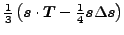
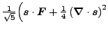
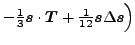
Table 21:
Spherical and Cartesian representations of
local densities (24) up to NLO. Only scalar
densities and the  components of vector densities are shown.
Numbers in the first column refer to numbers of primary densities
(23) shown in Tables 3 and
4. The last column shows factors preceding
densities in the Cartesian representation evaluated for
the phase conventions of Eq. (92). Time-even
densities are marked by using the bold-face font.
components of vector densities are shown.
Numbers in the first column refer to numbers of primary densities
(23) shown in Tables 3 and
4. The last column shows factors preceding
densities in the Cartesian representation evaluated for
the phase conventions of Eq. (92). Time-even
densities are marked by using the bold-face font.
| No. |
 |
|
|
|
|
Cartesian representation [25,30,24] |
Phase |
| 1 |
 |
= |
![$ [ \rho ]_{00}$](img693.png) |
= |
 |
 |
 |
| |
 |
= |
![$ [\nabla \rho ]_{10}$](img697.png) |
= |
 |
 |
 |
| |
 |
= |
![$ [[\nabla\nabla]_0\rho ]_{00}$](img702.png) |
= |
 |
 |
|
| 2 |
 |
= |
![$ [k \rho ]_{10}$](img706.png) |
= |
 |
 |
|
| |
 |
= |
![$ [\nabla[k \rho]_1]_{00}$](img710.png) |
= |
 |
 |
|
| |
 |
= |
![$ [\nabla[k \rho]_1]_{10}$](img714.png) |
= |
 |
 |
|
| 3 |
 |
= |
![$ [[kk]_{0} \rho ]_{00}$](img718.png) |
= |
 |
 |
|
| 17 |
 |
= |
![$ [ s ]_{10}$](img722.png) |
= |
 |
 |
|
| |
 |
= |
![$ [\nabla s ]_{00}$](img726.png) |
= |
 |
 |
|
| |
 |
= |
![$ [\nabla s ]_{10}$](img730.png) |
= |
 |
 |
|
| |
 |
= |
![$ [[\nabla\nabla]_0 s ]_{10}$](img734.png) |
= |
 |
 |
|
| |
 |
= |
![$ [[\nabla\nabla]_2 s ]_{10}$](img738.png) |
= |
|
 |
|
| 18 |
 |
= |
![$ [k s ]_{00}$](img741.png) |
= |
 |
 |
|
| |
 |
= |
![$ [\nabla[k s]_0]_{10}$](img745.png) |
= |
 |
 |
|
| 19 |
 |
= |
![$ [k s ]_{10}$](img749.png) |
= |
 |
 |
|
| |
 |
= |
![$ [\nabla[k s]_1]_{00}$](img753.png) |
= |
 |
 |
|
| |
 |
= |
![$ [\nabla[k s]_1]_{10}$](img757.png) |
= |
|
 |
|
| 21 |
 |
= |
![$ [[kk]_{0} s ]_{10}$](img760.png) |
= |
 |
 |
|
| 22 |
 |
= |
![$ [[kk]_{2} s ]_{10}$](img764.png) |
= |
|
 |
|
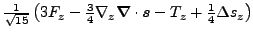
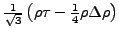
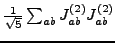
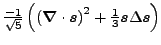
Table 22:
Spherical and Cartesian representations of
terms in the EDF (30) up to NLO. The
last column shows factors preceding terms in the Cartesian
representation evaluated using the phase conventions of
Eq. (92). Integration by parts was used to
transform
 into
into
 , which is the term used previously
in Refs. [30,24]. Coupling constants corresponding to terms
that depend on time-even densities are marked by using the bold-face
font. Bullets (
, which is the term used previously
in Refs. [30,24]. Coupling constants corresponding to terms
that depend on time-even densities are marked by using the bold-face
font. Bullets ( ) mark coupling constants corresponding to
terms that do not vanish for conserved spherical, space-inversion,
and time-reversal symmetries, see Sec. 4.
) mark coupling constants corresponding to
terms that do not vanish for conserved spherical, space-inversion,
and time-reversal symmetries, see Sec. 4.
| No. |
|
 |
|
![$ {[}\rho_{n'L'v'J'}{[}D_{mI} \rho_{nLvJ}{]}_{J'}{]}_0$](img769.png) |
|
 |
 Cartesian representation Cartesian representation |
Phase |
| 1 |
|
 |
|
![$ {[}\rho \rho {]}_0$](img772.png) |
= |
 |
 |
+1 |
| 2 |
|
 |
|
![$ {[}s s {]}_0$](img776.png) |
= |
 |
 |
+1 |
| 3 |
|
 |
|
![$ {[}\rho {[}{[}\nabla\nabla{]}_0 \rho {]}_0{]}_0$](img780.png) |
= |
 |
 |
+1 |
| 4 |
|
 |
|
![$ {[}\rho {[}{[}kk{]}_0\rho{]}_0 {]}_0$](img784.png) |
= |
 |
 |
+1 |
| 5 |
|
 |
|
![$ {[}{[}ks {]}_0 {[}k s{]}_0 {]}_0$](img788.png) |
= |
 |
 |
+1 |
| 6 |
|
 |
|
![$ {[}{[}ks {]}_1 {[}k s{]}_1 {]}_0$](img792.png) |
= |
|
 |
+1 |
| 7 |
|
 |
|
![$ {[}{[}ks {]}_2 {[}k s{]}_2 {]}_0 $](img795.png) |
= |
|
 |
+1 |
| 8 |
|
 |
|
![$ {[}\rho {[}\nabla {[}k s{]}_1{]}_0{]}_0$](img798.png) |
= |
 |
 |
+1 |
| 9 |
|
 |
|
![$ {[}{[}k\rho{]}_1 {[}k \rho{]}_1 {]}_0$](img802.png) |
= |
|
 |
+1 |
| 10 |
|
 |
|
![$ {[}s {[}{[}\nabla\nabla{]}_0 s {]}_1{]}_0$](img805.png) |
= |
 |
 |
+1 |
| 11 |
|
 |
|
![$ {[}s {[}{[}\nabla\nabla{]}_2 s {]}_1{]}_0$](img809.png) |
= |
|
 |
+1 |
| 12 |
|
 |
|
![$ {[}s {[}{[}kk{]}_0 s{]}_1 {]}_0$](img812.png) |
= |
|
 |
+1 |
| 13 |
|
 |
|
![$ {[}s {[}{[}kk{]}_2 s{]}_1 {]}_0$](img815.png) |
= |
|
 |
|
| |
|
|
|
|
|
|
 |
+1 |
| 14 |
|
 |
|
![$ {[}{[}k\rho{]}_1{[}\nabla s {]}_1{]}_0$](img819.png) |
= |
|
 |
+1 |
Among many options of choosing the phase convention, in the present
study we set
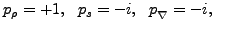 and and |
(92) |
This choice is unique in the fact that all scalar densities and all
terms in the EDF are then characterized by phase factors connecting
the spherical and Cartesian representations, see the last columns in
Tables 21 and 22. This allows for the closest
possible relationships between both representations, which may
facilitate the use of the spherical representation as it is
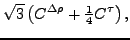
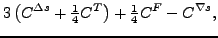
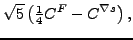
introduced in the present study. In particular, relations between
coupling constants up to NLO (Table 22) and standard
coupling constants in the Cartesian representation [24]
then read, for terms depending on time-even densities:
 |
 |
 |
(93) |
 |
|
 |
(94) |
 |
|
 |
(95) |
 |
|
 |
(96) |
 |
|
 |
(97) |
 |
|
 |
(98) |
 |
|
 |
(99) |
and for terms depending on time-odd densities:
 |
|
 |
(100) |
 |
|
 |
(101) |
 |
|
 |
(102) |
 |
|
 |
(103) |
 |
|
 |
(104) |
 |
|
 |
(105) |
 |
|
 |
(106) |
At the same time, all vector densities in Table 21 and
vector operators in Eqs. (89)-(91) are
consistently characterized by phase factors connecting the spherical
and Cartesian representations.
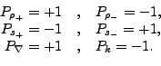
Phase conventions (92) also lead to very simple phase
properties, which our spherical tensors have with respect to complex
conjugation. Indeed, spherical tensors (88)-(91)
obey standard transformation rules under complex conjugation
[26],
 |
(107) |
where  . For nonlocal densities
(88)-(89), Eq. (107) holds separately
for their time-even and time-odd parts, split as in
Eqs. (63) and (64).
Using Eqs. (82) we then
have
. For nonlocal densities
(88)-(89), Eq. (107) holds separately
for their time-even and time-odd parts, split as in
Eqs. (63) and (64).
Using Eqs. (82) we then
have
 |
(108) |
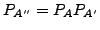
which for the phase convention of Eq. (92) reads
 |
(109) |
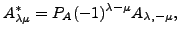
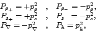
Standard rule (107) propagates through the angular
momentum coupling, i.e., if signs  and
and  characterize tensors
  and
and
 , respectively,
then the coupled tensor,
, respectively,
then the coupled tensor,
![$\displaystyle A''_{\lambda''\mu''} = [A_\lambda A'_{\lambda'}]_{\lambda''\mu''}...
...'} C^{\lambda''\mu''}_{\lambda\mu\lambda'\mu'} A_{\lambda\mu}A'_{\lambda'\mu'},$](img859.png) |
(110) |
is characterized by the product of signs
 .
Therefore, coupled higher-order densities (24) are
characterized by signs,
.
Therefore, coupled higher-order densities (24) are
characterized by signs,
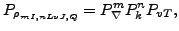 |
(111) |
where  or 1 denotes the scalar or vector density, or
  ,
respectively, and
,
respectively, and  or
or  denotes the time-even or time-odd density.
However, symmetry conditions (82) require that powers
of the
denotes the time-even or time-odd density.
However, symmetry conditions (82) require that powers
of the  derivative determine the time-reversal symmetry
of each local density, so that
derivative determine the time-reversal symmetry
of each local density, so that
 .
From Eqs. (108) we then obtain
.
From Eqs. (108) we then obtain
 |
(112) |
which for the phase convention of Eq. (92) reads
 |
(113) |
for all densities.
Therefore, the phase convention of Eq. (92) ensures
that scalar densities and all terms in the EDF are always real.
Next: Results for the Galilean
Up: Local nuclear energy density
Previous: Symmetry-covariant energy density
Jacek Dobaczewski
2008-10-06