Overview of the method

This introductory section is intended as a guide to the subsequent sections, where more detailed derivations and results are presented. Here, we use abbreviated notations so as to give a brief outline of the method, while referring the reader to the following sections for details.

The mean-field eigenvalue equation is obtained by considering the variation of the energy with the condition of the single-particle wavefunctions $\phi_{i}\left(\vec{r},\sigma\right)$ to be normalized to unity,

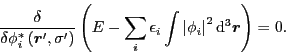$$\frac{\delta}{\delta\phi_{i}^{*}\left(\vec{r}',\sigma'\right... ...int\left\vert\phi_{i}\right\vert^{2}{\rm d}^3\vec{r}\right)=0.$$ (1)

The potential energy is expressed as the EDF of Ref. [4], that is,

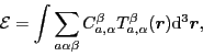$${\cal E}=\int\sum_{a\alpha\beta}C_{a,\alpha}^{\beta}T_{a,\alpha}^{\beta}(\vec{r}){\rm d}^3\vec{r},$$ (2)

where the grouped indices, such as the greek indices $\alpha=\left\{ n_{\alpha}L_{\alpha}v_{\alpha}J_{\alpha}\right\}$ or $\beta=\left\{ n_{\beta}L_{\beta}v_{\beta}J_{\beta}\right\}$ and the roman indices $a=\left\{m_aI_a\right\}$, denote all the quantum numbers of the local primary $\rho_{\beta}(\vec{r})$ and secondary $\rho_{a,\alpha,J}(\vec{r})$ densities [4]. In Eq. 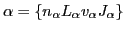(2), $T_{a,\alpha}^{\beta}(\vec{r})$ denotes terms of the functional,

$$T_{a,\alpha}^{\beta} \equiv \left[\rho_{\beta}\rho_{a,\alpha... ...L_{\alpha}v_{\alpha}J_{\alpha}}\right]_{J_{\beta}}\right]_{0},$$ (3)

$C_{a,\alpha}^{\beta}$ denote the coupling constants, $D_{a}$ denote the higher order derivative operators [4], and the sum runs over all terms of the functional. Although not shown explicitly the sum contains both isoscalar and isovector terms. At present we have neglected neutron-proton mixing which means that only the 0-component of the isovector densities are present. The convention adopted is such that the isovector contribution to the densities are taken as neutron minus proton densities and isoscalar densities are sums of neutron and proton densities.

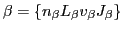
For each term of the functional, the variation with respect to the local densities, followed by the integration by parts and recoupling gives,

$$\delta\int T_{a,\alpha}^{\beta}{\rm d}^3\vec{r}=\int\left(\l... ...{\beta}\right]_{J_{\alpha}}\right]_{0}\right){\rm d}^3\vec{r},$$ (4)

cf. Eqs. (43) and (44). The primary densities can be expressed in terms of the single-particle wavefunctions as:

$$\rho_{nLvJ}=\left\{\left[K_{nL}\sum_{i\sigma\sigma'}\phi_{i}... ...vec{r}',\sigma'\right)\right]_{J}\right\}_{\vec{r}'=\vec{r}} .$$ (5)

The higher order derivative operators $K_{nL}$ [4] are built by coupling the relative-momentum operators $\vec{k}=\frac{1}{2i}\left(\vec{\nabla}^{\phi}-\vec{\nabla}^{\phi^{*}}\right)$, where we have used the subscripts to indicate on which function the operators act upon. This allows us to perform the variation with respect to $\phi_{i}^{*}$,

$$\frac{\delta}{\delta\phi_{i}^{*}}\int T_{a,\alpha}^{\beta}{\rm d}^3\vec{r} = \left[\left[K'_{n_{\beta}L_{\beta}}\sigma_{v_{\beta}}\phi_{i}\right]_{J_{\alpha}}\left[D_{a}\rho_{\alpha}\right]_{J_{\alpha}}\right]_{0}$$

$$+ \left(-1\right)^{J_{\beta}-J_{\alpha}}\left[\left[K'_{n_{\alpha}L... ...hi_{i}\right]_{J_{\beta}}\left[D_{a}\rho_{\beta}\right]_{J_{\beta}}\right]_{0}.$$ (6)

After performing the variation, the integral above was partially integrated so that the derivatives would not act on the variation of $\phi_{i}^{*}$. Therefore, the $K'_{nL}$ operators are built by coupling the relative-momentum operators $\vec{k}'=\frac{1}{2i}\left(\vec{\nabla}^{\phi}+\vec{\nabla}\right)$, where $\vec{\nabla}$ acts on all the functions of position standing to the right.

The operator on the right-hand-side of Eq. (6) is a formal expression for the mean-field operator. All what remains to be done is to disentangle the gradients $\vec{\nabla}^{\phi}$ and $\vec{\nabla}$ from one another - this procedure is performed in Eqs. (55)-(61) below. Finally, the mean-field operator $h\left(\rho\right)$ acquires the form:

$$h\left(\rho\right) =\sum_{\gamma}\left[U_{\gamma}\left[D_{n_\gamma L_\gamma}\sigma_{v_\gamma}\right]_{J_\gamma}\right]_{0},$$ (7)

where the differential operators $D_{n_\gamma L_\gamma}$ and Pauli matrices $\sigma_{v_\gamma}$ act on the single-particle wave functions, and the potentials $U_{\gamma}(\vec{r})$ are linear combinations of the secondary densities:

$$U_{\gamma}=\sum_{a\alpha\beta;d\delta}C_{a,\alpha}^{\beta}\c... ...}^{\beta;d\delta} \left[D_{d}\rho_{\delta}\right]_{J_\gamma}.$$ (8)

The coefficients $\chi_{a,\alpha;\gamma}^{\beta;d\delta}$ can be derived by using the recoupling rules presented in Section 3.3. An alternative method, which was also used when building the code HOSPHE (v1.00), was to construct the fields by starting from Eq. (6) and putting them equal to those of Eq. (7). This gives a linear system of equations that can be solved for the unknown coefficients $\chi_{a,\alpha;\gamma}^{\beta;d\delta}$. At N$^3$LO, only 1494 such coefficients are needed, so they can easily be precalculated and stored.

It is now clear, that the key operators in the mean field are given by

$$F_{d\delta,\gamma} =\left[\left[\rho_{d,\delta}\right]_{J_\g... ...gamma L_\gamma}\sigma_{v_\gamma}\right]_{J_\gamma}\right]_{0},$$ (9)

and their matrix elements in the single-particle basis $\phi_{i}\left(\vec{r},\sigma\right)$ read,

$$F^{ii'}_{d\delta,\gamma} = \langle\phi_{i}\vert F_{d\delta,\gamma}\vert\phi_{i'}\rangle$$

$$= \int\sum_{\sigma\sigma'} \phi_{i}^*\left(\vec{r},\sigma\right) \l... ..._{i'}\left(\vec{r},\sigma'\right)\right]_{J_\gamma}\right]_{0}{\rm d}^3\vec{r}.$$ (10)

Then, the mean-field matrix elements can be written as the following sum:

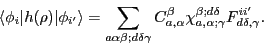$$\langle\phi_{i}\vert h(\rho)\vert\phi_{i'}\rangle =\sum_{a\... ...i_{a,\alpha;\gamma}^{\beta;d\delta} F^{ii'}_{d\delta,\gamma}.$$ (11)

Matrix elements in a spherical basis are derived in Sections 4.4 and 4.5.

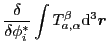
When constructing potentials (8), we need expressions to calculate all secondary densities. These can be written as [see Eqs. (76)-(78)]:

$$\rho_{d,\delta,JM} \equiv \left[D_{d}\rho_{\delta}\right]_{J... ...\sum_{bb'W}A_{d,\delta,J}^{bb',W}\rho_{v_{\delta}JM}^{bb',W} ,$$ (12)

with

$$\rho_{v_{\delta}JM}^{bb',W}\left(\vec{r}_{1}\right) =\left\{... ...\right)\right]_{JM}\right\}_{\vec{r}=\vec{r}_{2}=\vec{r}_{1}},$$ (13)

where the superscripts on the derivative operators indicate on which coordinate they act. The coefficients $A$ can be obtained by explicitly constructing the left- and right-hand sides of Eq. (12), which gives a linear system of equations in derivatives of the density matrix that can be solved for the unknown coefficients $A_{d,\delta,J}^{bb',W}$. At N$^3$LO, only 3138 such coefficients are needed, so they can easily be precalculated and stored. In Section 3.6 we also show how to derive these coefficients by using the recoupling rules and in Section 4.2 we give the expressions for densities in the spherical HO basis.