Conserved and Broken Symmetries

Representation of many-fermion states by density matrices (59) and (60), and the HF approximation of the two-body density matrix (69), allow us to give a precise definition of what one really means by conserved and broken symmetries in many-body systems. Moreover, it also links the spontaneous symmetry breaking mechanism to a description of correlations.

Consider a unitary symmetry operator $\hat P$ such that

$$\hat P^+ a_x\hat P = P_{xy}a_y \quad , \quad \hat P^+a^+_x\hat P = P_{xy}^{{\displaystyle \ast}}a^+_y$$ (76)

and

$$P^+_{xx'}T_{x'y'}P_{y'y} = T_{xy} \quad , \quad P^+_{zz'}P^+_{tt'}G_{z't'x'y'}P_{x'x}P_{y'y} = G_{ztxy} .$$ (77)

Equations (76) and (77) are equivalent to the symmetry condition $[\hat{H},\hat{P}]$=0 obeyed by Hamiltonian (57). Symmetry operator $\hat{P}$ acts in the fermion Fock space by mixing elementary fields $a^+_y$ with the integral kernel $P_{xy}$ (remember that the sum-integral ${\textstyle\int\hspace{-1.0em}\sum}{\rm d}{y}$ is implied for every repeated index). All the most interesting symmetries act in this way - they can be represented as exponents of one-body symmetry generators, i.e., $\hat{P}$ can be any one of the following:

1egintex2html_wrap_inlinecircendtex2html_wrap_inline.

translational symmetry,

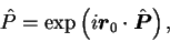$$\hat{P} = \exp\left(i\mbox{{\boldmath {$r$}}}_0\cdot\hat{\mbox{{\boldmath {$P$}}}}\right),$$ (78)

where $\hat{\mbox{{\boldmath {$P$}}}}$= $\sum_{i=1}^A \mbox{{\boldmath {$p$}}}_i$ is the total linear momentum operator, and $\mbox{{\boldmath {$r$}}}_0$ is the shift vector.

2egintex2html_wrap_inlinecircendtex2html_wrap_inline.

rotational symmetry,

$$\hat{P} = \exp\left(i\mbox{{\boldmath {$\alpha$}}}_0\cdot\hat{\mbox{{\boldmath {$I$}}}}\right),$$ (79)

where $\hat{\mbox{{\boldmath {$I$}}}}$= $\sum_{i=1}^A \mbox{{\boldmath {$j$}}}_i$ is the total angular momentum operator, and $\mbox{{\boldmath {$\alpha$}}}_0$ is the rotation angle.

3egintex2html_wrap_inlinecircendtex2html_wrap_inline.

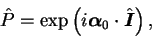
isospin symmetry,

$$\hat{P} = \exp\left(i\vec{\alpha}_0\circ \hat{\vec{T}}\right),$$ (80)

where $\hat{\vec{T}}$= ${\textstyle{\frac{1}{2}}}\sum_{i=1}^A \vec{\tau}_i$ is the total isospin operator, and $\vec{\alpha}_0$ is the iso-rotation angle.

4egintex2html_wrap_inlinecircendtex2html_wrap_inline.

particle-number symmetry,

$$\hat{P} = \exp\left(i\phi_0\hat{N}\right),$$ (81)

where $\hat{N}$= ${\textstyle\int\hspace{-1.0em}\sum}{\rm d}{x}\,a^+_xa_x$ is the total particle number operator, and $\phi_0$ is the gauge angle.

5egintex2html_wrap_inlinecircendtex2html_wrap_inline.

inversion (parity) symmetry,

$$\hat{P} = \prod_{i=1}^A\,\hat{\pi}_i,$$ (82)

where $\hat{\pi}_i$ is the inversion operator for the $i$th particle.

6egintex2html_wrap_inlinecircendtex2html_wrap_inline.

time-reversal symmetry.

$$\hat{P} = \exp\left(-i\pi \hat{S}_y\right)\hat{K} ,$$ (83)

where $\hat{S}_y$= ${\textstyle{\frac{1}{2}}}\sum_{i=1}^A \sigma_{iy}$ is the $y$ component of the total spin operator, and $\hat{K}$ is the complex conjugation operator in spatial representation.

There can also be terms in the Hamiltonian that explicitly break some of the above symmetries (e.g., the Coulomb interaction explicitly breaks the isospin symmetry), but we disregard them for simplicity.

Let us begin with the simplest case, namely, let $\hat{P}$ be the parity symmetry (82). In this case, the integral kernel reads $P_{xy}$$\equiv$ $\delta(\mbox{{\boldmath {$x$}}}+\mbox{{\boldmath {$y$}}})$, and is, of course, independent of spin and isospin. For a parity-invariant interaction, Eq. (77), the exact energy of an arbitrary state $\vert\Psi\rangle$, Eq. (58), depends only on the scalar parts (in this case, the parity invariant parts) of the one- and two-body density matrices, i.e.,

$$E = T_{xy}\rho_{yx}^{(+)} + {\textstyle{\frac{1}{4}}}G_{xyzt}\rho_{ztxy}^{(+)} ,$$ (84)

for

$$\rho_{yx}^{(\pm)} = {\textstyle{\frac{1}{2}}}\left(P_{yy'}\rho_{y'x'}P^+_{x'x} \pm \rho_{yx}\right) ,$$ (85)

$$\rho_{ztxy}^{(\pm)} = {\textstyle{\frac{1}{2}}}\left(P_{zz'}P_{tt'}\rho_{z't'x'y'} P^+_{x'x}P^+_{y'y} \pm \rho_{ztxy}\right) .$$ (86)

Within the HF approximation (69), we may have two classes of solutions:

• symmetry-conserving solution:
  

  $$\rho_{xy} = \rho_{xy}^{(+)} ,$$ (87)

  $$\rho_{ztxy}^{(+)} = \rho_{zx}^{(+)}\rho_{ty}^{(+)} - \rho_{zy}^{(+)}\rho_{tx}^{(+)} ,$$ (88)

  
  

• symmetry-breaking solution:
  

  $$\rho_{xy} = \rho_{xy}^{(+)} + \rho_{xy}^{(-)} ,$$ (89)

  $$\rho_{ztxy}^{(+)} = \rho_{zx}^{(+)}\rho_{ty}^{(+)} - \rho_{zy}^{(+)}\rho_{tx}^{(+)} + \rho_{zx}^{(-)}\rho_{ty}^{(-)} - \rho_{zy}^{(-)}\rho_{tx}^{(-)} .$$ (90)

  
  

In the case of the broken symmetry, neither of the density matrices is invariant with respect to the symmetry operator. However, the symmetry breaking part of the one-body density matrix $\rho_{xy}^{(-)}$ enters the HF energy (84) only through the two-body interaction energy. Moreover, the symmetry-projected two-body density matrix (90) does not obey the HF condition (69). In other words, the symmetry-breaking part of the one-body density matrix gives a correlation term of the two-body density matrix. Symmetry breaking is, therefore, a reflection of correlations beyond HF, taken into account with respect to the symmetry-conserving HF method.

One can also say that the symmetry-breaking part $\rho_{xy}^{(-)}$ constitutes an additional set of variational parameters, which become allowed when a larger class of the one-body density matrices (beyond symmetry conservation) is considered. As in every variational procedure, a larger variational class may lead (sometimes) to lower energies. Whether it does, depends on the specific case, and in particular on the type of the two-body interaction. It is obvious, that one can gain energy by breaking symmetry only if the appropriate correlation energy is negative, i.e., when the last two terms of the two-body density matrix, $\rho_{zx}^{(-)}\rho_{ty}^{(-)} - \rho_{zy}^{(-)}\rho_{tx}^{(-)}$, give a negative contribution when averaged with the two-body effective interaction $G_{xyzt}$.

Within such an approach to the symmetry breaking, one does not, in fact, break any symmetry of the exact wave function. Indeed, the density matrices, $\rho_{xy}^{(+)}$ and $\rho_{ztxy}^{(+)}$ that are ``active'' in the total energy do conserve the symmetry. We should also use these density matrices to calculate all other observables for the symmetry-broken (correlated) solution of the HF equations.

Let us now give results of an analogous analysis for the case of deformed nuclei, i.e., for the case of broken rotational symmetry (79). For axial shapes we then have the following density matrices,

$$\rho_{xy} = \sum_{J}\rho_{xy}^{(J)} ,$$ (91)

$$\rho_{ztxy}^{(0)} = \sum_{J}\left(\rho_{zx}^{(J)}\times\rho_{ty}^{(J)}\right)_{0} - \sum_{J}\left(\rho_{zy}^{(J)}\times\rho_{tx}^{(J)}\right)_{0} ,$$ (92)

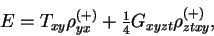
and the total HF energy,

$$E = T_{xy}\rho_{yx}^{(0)} + {\textstyle{\frac{1}{4}}}G_{xyzt}\rho_{ztxy}^{(0)} ,$$ (93)

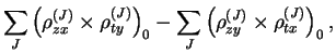
that depends only on the scalar ($J$=0) parts of the density matrices. On the other hand, the broken-symmetry one-body density matrix is the sum of components $\rho_{xy}^{(J)}$ that transform as irreducible rotational tensors of rank $J$. In the scalar two-body density matrix (92), these components are coupled to $J$=0, and every such a term defines the multipole correlation energy of rank $J$. It is now obvious that the broken-symmetry solution becomes the ground state for interactions that have appropriately strong multipole-multipole terms (see Refs. Dob88,Wer94 for numerical results in heavy nuclei).

Figure 10: Schematic illustration of the s.p. level density (left), corresponding to the s.p. spectrum of a deformed nucleus (centre). The right panel shows the evolution of the spectrum with nuclear deformation. (Picture courtesy: W. Nazarewicz, ORNL/University of Tennessee/Warsaw University.) From http://www-highspin.phys.utk.edu/~ witek/.

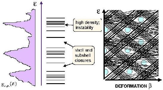Without going into detailed discussion of the multipole-multipole decomposition of effective interactions, we may easily tell in which nuclei the rotational symmetry is broken and deformation appears. A schematic diagram presented in the right panel of Fig. 10 shows the evolution of the s.p. spectrum with nuclear deformation, i.e., the dependence of eigenvalues of the mean-field Hamiltonian having the shape characterized by the deformation parameter $\beta$. In such a spectrum, some s.p. levels go down, and other go up in energy, and at specific deformations there appear in the spectrum larger or smaller gaps. When the particles are filling the lowest levels up to certain energy (prescribed by the number of particles), the last occupied level may appear either below or above the gap. This leads respectively to a decrease or an increase of the total energy. The overall density of s.p. levels at the Fermi surface determines, therefore, the total energy of the system. In other words, a system having a given number of particles adopts the shape at which the last occupied level is below a large gap. Therefore, nuclei that correspond to magic particle numbers are spherical (large gaps appear at spherical shape) and the rotational symmetry is conserved, while nuclei with particle numbers between the magic gaps (the so-called open-shell nuclei) choose non-zero deformed ground states corresponding to broken rotational symmetry.