Approximation of the many-body energy (58) by a functional of the one-body density matrix (70) can be further simplified in the coordinate representation. Namely, it appears that the HF density matrix (75) influences the energy mostly through the local density Neg70,Neg72,Neg75. This observation defines the local density approximation (LDA).
Neglecting for simplicity the spin-isospin
degrees of freedom, we can write the
interaction energy [the second term in Eq. (70)]
in the form
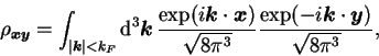
It is therefore convenient to represent the one-body density
matrix (59) in total and relative coordinates, i.e.,
In the direct term, we can use the fact that the range of the
effective force is smaller than the typical distance at which the
density changes. Indeed, the nuclear density is almost constant
inside the nucleus, and then falls down to zero within the region
called the nuclear surface, which has a typical width of about 3fm.
Hence, within the range of interaction, and for the purpose of
evaluating the direct interaction energy, the density can be
approximated by the quadratic expansion,
In the exchange term, the situation is entirely different, because
here the range of interaction matters in the non-local, relative
direction
![]() . In order to get a feeling what are the properties
of the one-body density matrix in this direction, we can calculate it
for infinite matter,
. In order to get a feeling what are the properties
of the one-body density matrix in this direction, we can calculate it
for infinite matter,
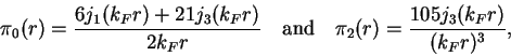
Therefore, the quadratic expansion of the density matrix in the
relative variable
The term depending on the non-local density in the exchange integral
(99) now reads
Altogether, quadratic approximations to the one-body density matrix allow expressing the direct and exchange interaction energies as integrals of local energy density. Such energy density depends on the local density, on derivatives of the local density, and on several other densities that represent properties of the one-body density matrix in the non-local direction.
We should stress that the validity of the LDA depends on different scales involved in properties of nuclei. Namely, the scale of distances characterizing the ground-state one-body density matrix is significantly larger than the range of effective forces. Therefore, the LDA may apply only to selected, low-energy phenomena where the spatial structure of the density matrix is not very much affected.
Moreover, we see that the low-energy nuclear properties may depend on an extremely restricted set of properties of effective interactions. Within the LDA, only a few numbers [the coupling constants of Eqs. (103) and (113)] determine the energy density. This is entirely in the spirit of the effective field theory; separation of scales results in a transmission of a very limited information from one scale to another. Once this information (in our case - the coupling constants) is either evaluated, or fit to data, properties of the system can be properly calculated at the larger scale.
We also see that the coupling constants can be evaluated by assuming any effective interaction that has a smaller range than the physical range. In doing so, we can even go down to zero range, and nothing will change, provided we fix the parameters of the zero-range force so as to properly describe the moments of the force, Eqs. (103) and (113), and thus properly reproduce the coupling constants.
We can now proceed to the real world by putting back into our description the spin and isospin degrees of freedom. Based on the results above, we can first construct the most general set of local densities, with derivatives up to the second order taken into account, and then build the local energy density. The complete such construction has been performed only very recently Per03; it involves the full proton-neutron mixing and treats both the particle-hole and particle-particle channels of interaction.
We begin by writing the one-body density matrix (59)
with all variables shown explicitly,
Without the proton-neutron mixing, which we neglect from now on in
order to simplify the presentation, only the third components of
isovectors are non-zero, and we can use the notation
For an arbitrary central finite-range local potential with the full
spin-isospin dependence [cf. the Gogny interaction in Eq. (63)],
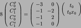
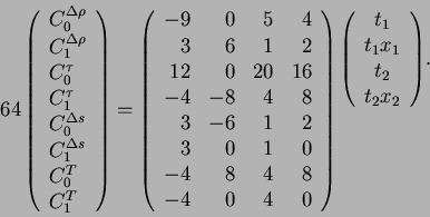
 . The energy density depends
on six isoscalar and six isovector coupling constants that are
simple moments of potentials, i.e.,
. The energy density depends
on six isoscalar and six isovector coupling constants that are
simple moments of potentials, i.e.,
Again we see, that for
![]() , the
direct and exchange coupling constants are equal,
, the
direct and exchange coupling constants are equal, ![]() and
and
![]() , and hence only six coupling constants in energy density
(126) are independent. This requires that the so-called
time-odd coupling constants are linear combinations of the so-called
time-even coupling constants Dob95e:
, and hence only six coupling constants in energy density
(126) are independent. This requires that the so-called
time-odd coupling constants are linear combinations of the so-called
time-even coupling constants Dob95e:
It is well known that the local energy density (126) is also
obtained for the Skyrme zero-range momentum-dependent interaction
Sky56,Sky59,Vau72. Without density-dependent
and spin-orbit terms, this interaction reads
Again we explicitly see that (exactly in the spirit of the effective field theory), the zero-range interaction can reproduce the same properties of nuclear systems as does the real effective interaction, provided the coupling constants in the energy density are either adjusted to data, or calculated from the real finite-range interaction. It is also clear that the zero-range interaction cannot be treated literally - it is significant only as a ``generator'' of the proper energy density, while all physical results depend only on this energy density, and not on the interaction itself. In particular, it is incorrect to look for exact eigenstates of the system interacting with the zero-range interaction; we know that for such an interaction the ground state does not exist because of the collapse. However, even for the finite-range effective interaction (for which the ground state does, in principle, exist) the exact ground state is irrelevant, because the interaction has been built to act only in the space of Slater determinants, see Sec. 4.2.
Of course, there is nothing magic or fundamental in the LDA to the energy density. It just reflects the fact that the nuclear one-body density matrix varies on a larger scale of distances than does the nuclear effective interaction. Validity of this approximation depends on the fundamental assumption that the total energy can be described as a functional of the one-body density matrix. The fact that we assumed a local effective interaction is not crucial - for non-local interactions the direct term becomes more complicated, but the LDA still holds Neg72. However, effective interactions must, in fact, also depend on energy (Secs. 4.2 and 4.3), so the presented derivation of the LDA is not complete. One usually goes beyond the local energy density derived from approximations to one-body density, and one includes also terms that depend on local densities in a more complicated way, cf. the density-dependent term of the Gogny interaction (63).
Some people say: the LDA is just fitting of parameters - it is enough to have many parameters to fit anything one wants. This point of view simply disregards the success of the LDA in nuclear phenomenology. The effective field theory point of view is, in my opinion, more interesting, and potentially more fruitful. It regards the success of phenomenological LDA as indication that scales between quark-gluon QCD interactions and low-energy nuclear phenomena are indeed very well separated, and hence few numbers only are enough to define latter in terms of the former. The challenge of course remains: to look for derivations of these few numbers by decent fundamental theory, and to adjust these numbers to data and look for phenomena where the adjustments fail.
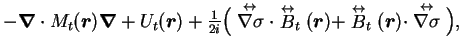
We finish this section by recalling the form of the HF equation
(73), and that of the HF mean-field Hamiltonian
(72), corresponding to the local-energy-density functional
(126). Upon variation of the energy with respect to local
densities, one obtains the HF equation (74) in spatial coordinates,
Bibliografia
[Mes71]A. Messiah, Méchanique Quantique (Paris, Masson et Cie, 1971).
[Lan70]L. Landau and E. Lifchitz, Théorie des Champs (Moscou, Mir, 1970).
[Wei99]S. Weinberg, The Quantum Theory of Fields (Cambridge University Press, Cambridge, 1996-2000) Vols. I-III.
[Jac75]J.D. Jackson, Classical Electrodynamics (Wiley, New York, 1975).
[Itz80]C. Itzykson and J.-B. Zuber, Quantum Field Theory (McGraw-Hill, New York, 1980).
[Hug99]V.W. Hughes and T. Kinoshita, Rev. Mod. Phys. 71, S133 (1999).
[Dyc87]R.S. Van Dyck Jr., P.B. Schwinberg, and H.G. Dehmelt, Phys. Rev. Lett. 59, 26 (1987).
[Gra95]W. Greiner and A. Schäfer, Quantum Chromodynamics (Berlin, Springer, 1995).
[Gil74]R. Gilmore, Lie grooups, Lie algebras and some of their applications (Wiley, New York, 1974).
[Plu86]G. Plunien, B. Müller, and W. Greiner, Phys. Rep. 134, 87 (1986).
[Lei00]D.B. Leinweber, hep-lat/0004025.
[Gel60]M. Gell-Mann and M. L'evy, Nuovo Cim. 16, 705 (1960).
[Wei67]S. Weinberg, Phys. Rev. Lett. 18, 188 (1967).
[Gol61]J. Goldstone, Nuovo Cim. 19, 154 (1961).
[Yuk35]H. Yukawa, Proc. Math. Soc. Japan 17, 48 (1935).
[Wir95]R.B. Wiringa, V.G.J. Stoks, and R. Schiavilla, Phys. Rev. C51, 38 (1995).
[Exu96]Antoine de Saint-Exupéry, Le Petit Prince (Paris, Gallimard, 1996).
[Lep97]G.P. Lepage, nucl-th/9706029.
[Ent02]D.R. Entem and R. Machleidt, Phys. Lett. B524, 93 (2002).
[Pie02]S.C. Pieper, K. Varga, and R.B. Wiringa, Phys. Rev. C66, 044310 (2002).
[Wir02]R.B. Wiringa and S.C. Pieper, Phys. Rev. Lett. 89, 182501 (2002).
[Pie01a]S.C. Pieper, V.R. Pandharipande, R.B. Wiringa, and J. Carlson, Phys. Rev. C64, 014001 (2001).
[Col63]A.J. Coleman, Rev. Mod. Phys. 35, 668 (1963).
[Col00]A.J. Coleman and V.I. Yukalov, Reduced Density Matrices: Coulson's Challenge (Springer-Verlag, New York, 2000).
[Fet71]A.L. Fetter and J.D. Walecka, Quantum Theory of Many-Particle Systems (McGraw-Hill, Boston, 1971).
[Hax00]W.C. Haxton and C.-L. Song, Phys. Rev. Lett. 84, 5484 (2000).
[Hax02]W.C. Haxton and T. Luu, Phys. Rev. Lett. 89, 182503 (2002).
[Gog75b]D. Gogny, in Nuclear Self-Consistent Fields, ed. G. Ripka and M. Porneuf (North-Holland, Amsterdam, 1975) p. 333.
[RS80]P. Ring and P. Schuck, The Nuclear Many-Body Problem (Springer-Verlag, Berlin, 1980).
[Blo58]C. Bloch and J. Horowitz, Nucl. Phys. bf 8, 91 (1958).
[Dob88]J. Dobaczewski, W. Nazarewicz, J. Skalski and T.R. Werner, Phys. Rev. Lett. 60, 2254 (1988).
[Wer94]T.R. Werner, J. Dobaczewski, M.W. Guidry, W. Nazarewicz, and J.A. Sheikh, Nucl. Phys. A578, 1 (1994).
[Neg70]J.W. Negele, Phys. Rev. C1, 1260 (1970).
[Neg72]J.W. Negele and D. Vautherin, Phys. Rev. C5, 1472 (1972).
[Neg75]J.W. Negele, Lecture Notes in Physics 40 (Springer, Berlin, 1975), pp. 285, 288.
[Dob95e]J. Dobaczewski and J. Dudek, Phys. Rev. C52, 1827 (1995); C55, 3177(E) (1997).
[Per03]E. Perlinska, S.G. Rohozinski, J. Dobaczewski, and W. Nazarewicz, to be published.
[Eng75]Y.M. Engel, D.M. Brink, K. Goeke, S.J. Krieger, and D. Vautherin, Nucl. Phys. A249, 215 (1975).
[Flo75]H. Flocard, Thesis 1975, Orsay, Série A, N![]() 1543.
1543.
[Sky56]T.H.R. Skyrme, Phil. Mag. 1, 1043 (1956).
[Sky59]T.H.R. Skyrme, Nucl. Phys. 9, 615 (1959).
[Vau72]D. Vautherin and D.M. Brink, Phys. Rev. C5, 626 (1972).
![\begin{displaymath}
\rho(\mbox{{\boldmath {$R$}}},\mbox{{\boldmath {$r$}}}) = \f...
...= \frac{k_F^3}{6\pi^2}\,\left[3\frac{j_1(k_Fr)}{k_Fr}\right] .
\end{displaymath}](img452.png)
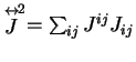
![\begin{displaymath}
{ E}^{\mbox{\scriptsize {int}}} = \sum_{t=0,1}{\displaystyl...
...oldmath {$T$}}}_t
- \stackrel{\leftrightarrow}{J}_t^2)\Big] ,
\end{displaymath}](img517.png)