Effective Interactions (I)

We saw that the crucial element of the dimensionality is the number of space-spin-isospin points needed to describe basic fields $a^+_x$. Therefore, we have to use methods that lead to fields as slowly varying in function of position, as it is possible. In this respect, region of the phase space that corresponds to pairs of nucleons getting near one another, is particularly cumbersome, because the wave functions must vary rapidly there, in order to become very small within the radius of the strong repulsion, cf. Fig. 5 above. In the past, very powerful technics have been developed to treat these hard-core effects. They are based on replacing the real NN interaction $V_{xyx'y'}$ by the effective interaction $G_{xyx'y'}$ that fulfills the following condition

$$\int\hspace{-1.2em}\sum {\rm d}{x'}{\rm d}{y'}\,V_{xyx'y'}\... ...)\phi_{j}(y') -\phi_{i}(y')\phi_{j}(x')}{\sqrt{2}}}}\right] ,$$ (61)

where the sum-integrals are performed over $x'$ and $y'$.

The two-body wave function in the square brackets on the r.h.s. is the independent-particle, or product wave function, built as the antisymmetrized product of two s.p. wave functions, $\phi_{i}(x)$ and $\phi_{j}(x)$, characterized by quantum numbers $i$ and $j$. The two-body wave function on the l.h.s., $\Psi_{ij}(x',y')$, is a wave function correlated at the short range; it is very small within the region of the hard core. So the real NN interaction, when acting on the correlated wave function, gives a finite result, because the wave function is very small in the region where the repulsion is vary large. On the other hand, the antisymmetrized product wave function is never small around $x'$=$y'$ (although it vanishes at $x'$=$y'$), and hence the effective interaction fulfilling (61) has no hard core. Condition (61) defines, therefore, the effective interaction that can be used in the space of uncorrelated Slater determinants. The whole procedure can be put on firm grounds in the framework of the perturbation expansion, when partial sums of infinite classes of diagrams are performed, but this is beyond the scope of the present lectures. We only mention that within such a formalism, the effective interaction is obtained by solving the Bethe-Goldstone equation Fet71.

The effective interaction should, in principle, depend on the s.p. states $\phi_{i}(x)$ and $\phi_{j}(x)$ for which the Bethe-Goldstone equation is solved. For example, the effective interaction in an infinite nuclear matter, where the s.p. wave functions are plane waves, can be different than that in a finite nucleus. In the past, there were many calculations pertaining to the first case, while the second (and more interesting) situation was successfully addressed only very recently Hax00,Hax02.

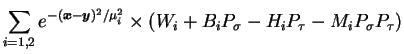
On a phenomenological level, one can postulate simple forms of interactions and use them as models of such difficult-to-derive effective interactions. Such a route was adopted by Gogny Gog75b, who postulated the simple local interaction

$$\tilde{G}_{xyx'y'} = \delta(\mbox{{\boldmath {$x$}}}-\mbox{{... ...(\mbox{{\boldmath {$y$}}}-\mbox{{\boldmath {$y$}}}') G(x,y) ,$$ (62)

where the tilde denotes a non-antisymmetrized matrix element ( ${G}_{xyx'y'} = \tilde{G}_{xyx'y'} - \tilde{G}_{xyy'x'}$), in the form of a sum of two Gaussians, plus a zero-range, density dependent part,²

$$G(x,y) = \sum_{i=1,2} e^{-(\mbox{{\boldmath {${\scriptstyle x}$}}}-\mbox{{... ...}$}}})^2/\mu^2_i}\times (W_i + B_i P_\sigma - H_i P_\tau - M_i P_\sigma P_\tau)$$

$$+ t_3(1+P_\sigma)\delta(\mbox{{\boldmath {$x$}}}-\mbox{{\boldmath {... ...style{\frac{1}{2}}}(\mbox{{\boldmath {$x$}}}+\mbox{{\boldmath {$y$}}})\right] .$$ (63)

In this Equation, $P_\sigma$= ${\textstyle{\frac{1}{2}}}(1$$+$ $\mbox{{\boldmath {$\sigma$}}}_1\cdot\mbox{{\boldmath {$\sigma$}}}_2)$ and $P_\tau$= ${\textstyle{\frac{1}{2}}}(1$$+$ $\vec{\tau}_1\circ \vec{\tau}_2)$ are, respectively, the spin and isospin exchange operators of particles 1 and 2, $\rho(\mbox{{\boldmath {$r$}}})$ is the total density of the system at point $\mbox{{\boldmath {$r$}}}$, and $\mu_i$, $W_i$, $B_i$, $H_i$, $M_i$, and $t_3$ are parameters.

Figure 8: Comparison of the Gogny and Argonne v$_{18}$ $n$-$n$ potentials in the $^3$S$_1$ (top) and $^1$S$_0$ (bottom) channels. Note very different scales of the top and bottom panels.

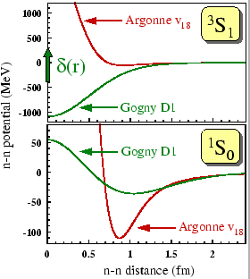In Fig. 8, we compare the real $n$-$n$ interaction (Argonne v$_{18}$) with the effective Gogny interaction (the D1 parametrization Gog75b,RS80) in the $L$=0 channels, i.e., in the $^3$S$_1$ channel ($P_\sigma$=1 and $P_\tau$=$-$1) and $^1$S$_0$ channel ($P_\sigma$=$-$1 and $P_\tau$=1). It is clear that real and effective interactions are very different near $\mbox{{\boldmath {$r$}}}$=0. The zero-range piece of the interaction acts only in the $^3$S$_1$ channel; in Fig. 8 it is represented by the green arrow at $\mbox{{\boldmath {$r$}}}$=0. One should keep in mind that the Gogny interaction is meant to represent the effective interaction, and hence it can only act on the product wave functions. In particular, an attempt to solve exactly, e.g., the two-body (deuteron) problem goes beyond the range of applicability of the effective interaction. The Gogny interaction is mostly used within the mean-field approximation that we discuss in more detail in the Sec. 4.4 below.