next up previous
Next: Skyrme interaction energy functional Up: The Energy Density Functional Previous: The Energy Density Functional


Local gauge invariance

Under a local gauge transformation [175], many body wave function is multiplied by position-dependent phase factor
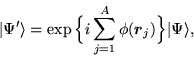
\begin{displaymath}
\vert\Psi'\rangle = \exp\Big\{i\sum_{j=1}^A\phi(\mbox{{\boldmath {$r$}}}_j)\Big\}
\vert\Psi\rangle,
\end{displaymath} (82)

which induces the following gauge transformations of density matrices (1) and (4),
$\displaystyle \hat{\rho}'(\mbox{{\boldmath {$r$}}}st,\mbox{{\boldmath {$r$}}}'s't')$ $\textstyle =$ $\displaystyle e^{i\phi(\mbox{{\boldmath {$r$}}})-i\phi(\mbox{{\boldmath {$r$}}}')}
\hat{\rho}(\mbox{{\boldmath {$r$}}}st,\mbox{{\boldmath {$r$}}}'s't'),$ (83)
$\displaystyle \hat{\breve{\rho}}'(\mbox{{\boldmath {$r$}}}st,\mbox{{\boldmath {$r$}}}'s't')$ $\textstyle =$ $\displaystyle e^{i\phi(\mbox{{\boldmath {$r$}}})+i\phi(\mbox{{\boldmath {$r$}}}')}
\hat{\breve{\rho}}(\mbox{{\boldmath {$r$}}}st,\mbox{{\boldmath {$r$}}}'s't').$ (84)

The Galilean transformation is a local gauge transformation for $\phi(\mbox{{\boldmath {$r$}}})$= $\mbox{{\boldmath {$p$}}}\cdot\mbox{{\boldmath {$r$}}}$, where $\mbox{{\boldmath {$p$}}}$ 
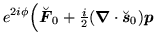
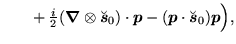
is a constant boost momentum. In analogy to that, one can introduce the local momentum field defined by
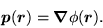
\begin{displaymath}
\mbox{{\boldmath {$p$}}}(\mbox{{\boldmath {$r$}}}) = \mbox{{\boldmath {$\nabla$}}}\phi(\mbox{{\boldmath {$r$}}}) .
\end{displaymath} (85)

Local and momentum-independent interaction is invariant with respect to local gauge transformation, and hence energy densities (78) and (80) must then also be independent of the local gauge. The question whether it is possible to model nuclear effective interactions in the p-h and p-p channels by a local and momentum-independent interaction, is open. Therefore, gauge transformation of the energy density can, in principle, be respected or not, depending on a choice of dynamics one makes.

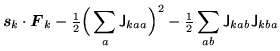
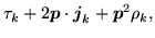
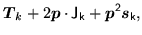
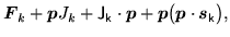
It is easy to tell when the local energy densities (78) and (80) are local-gauge invariant, because properties of local densities (38)-(50) under gauge transformation read explicitly

$\displaystyle \rho' _k\ofbboxofr $ $\textstyle =$ $\displaystyle \rho _k\ofbboxofr $ (86)
$\displaystyle \tau' _k\ofbboxofr $ $\textstyle =$ $\displaystyle \tau _k\ofbboxofr + 2\mbox{{\boldmath {$p$}}} \ofbboxofr\cdot\mbo...
...{$j$}}} _k\ofbboxofr + \mbox{{\boldmath {$p$}}}^2 \ofbboxofr\rho _k\ofbboxofr ,$ (87)
$\displaystyle \mbox{{\boldmath {$s$}}}' _k\ofbboxofr $ $\textstyle =$ $\displaystyle \mbox{{\boldmath {$s$}}} _k\ofbboxofr ,$ (88)
$\displaystyle \mbox{{\boldmath {$T$}}}' _k\ofbboxofr $ $\textstyle =$ $\displaystyle \mbox{{\boldmath {$T$}}} _k\ofbboxofr + 2\mbox{{\boldmath {$p$}}}...
... + \mbox{{\boldmath {$p$}}}^2 \ofbboxofr\mbox{{\boldmath {$s$}}} _k\ofbboxofr ,$ (89)
$\displaystyle \mbox{{\boldmath {$j$}}}' _k\ofbboxofr $ $\textstyle =$ $\displaystyle \mbox{{\boldmath {$j $}}}_k\ofbboxofr + \mbox{{\boldmath {$p$}}} \ofbboxofr\rho _k\ofbboxofr ,$ (90)
$\displaystyle \mbox{{\boldmath {$F$}}}' _k\ofbboxofr $ $\textstyle =$ $\displaystyle \mbox{{\boldmath {$F$}}} _k\ofbboxofr + \mbox{{\boldmath {$p$}}} ...
...{{\boldmath {$p$}}} \ofbboxofr\cdot\mbox{{\boldmath {$s$}}} _k\ofbboxofr\big) ,$ (91)
$\displaystyle \mathsf{J}'_k\ofbboxofr $ $\textstyle =$ $\displaystyle \mathsf{J}_k\ofbboxofr + \mbox{{\boldmath {$p$}}} \ofbboxofr\otimes\mbox{{\boldmath {$s$}}}_k\ofbboxofr ,$ (92)

where $k$=0,1,2,3, and
$\displaystyle \vec{\breve{\rho~}}' \ofbboxofr $ $\textstyle =$ $\displaystyle e^{2i\phi \ofbboxofr }
\vec{\breve{\rho}} \ofbboxofr $ (93)
$\displaystyle \vec{\breve{\tau~}}' \ofbboxofr $ $\textstyle =$ $\displaystyle e^{2i\phi \ofbboxofr }\big(
\vec{\breve{\tau}} \ofbboxofr + i\mbo...
...ofr - \mbox{{\boldmath {$p$}}}^2 \ofbboxofr\vec{\breve{\rho}} \ofbboxofr\big) ,$ (94)
$\displaystyle \breve{\mbox{{\boldmath {$s$}}}}' _0\ofbboxofr $ $\textstyle =$ $\displaystyle e^{2i\phi \ofbboxofr }
\breve{\mbox{{\boldmath {$s$}}}} _0\ofbboxofr ,$ (95)
$\displaystyle \breve{\mbox{{\boldmath {$T$}}}}' _0\ofbboxofr $ $\textstyle =$ $\displaystyle e^{2i\phi \ofbboxofr }\big(
\breve{\mbox{{\boldmath {$T$}}}} _0\o...
...ldmath {$p$}}}^2 \ofbboxofr\breve{\mbox{{\boldmath {$s$}}}} _0\ofbboxofr\big) ,$ (96)
$\displaystyle \breve{\mbox{{\boldmath {$j$}}}}' _0\ofbboxofr $ $\textstyle =$ $\displaystyle e^{2i\phi \ofbboxofr }
\breve{\mbox{{\boldmath {$j$}}}} _0\ofbboxofr ,$ (97)
$\displaystyle \breve{\mbox{{\boldmath {$F$}}}}' _0\ofbboxofr $ $\textstyle =$ $\displaystyle e^{2i\phi \ofbboxofr }\Big(
\breve{\mbox{{\boldmath {$F$}}}} _0\o...
...e{\mbox{{\boldmath {$s$}}}} _0\ofbboxofr )
\mbox{{\boldmath {$p$}}} \ofbboxofr $  
    $\displaystyle ~~~~~
+ {\textstyle{\frac{i}{2}}}(\mbox{{\boldmath {$\nabla$}}}\o...
...x{{\boldmath {$s$}}}} _0\ofbboxofr )
\mbox{{\boldmath {$p$}}} \ofbboxofr\Big) ,$ (98)
$\displaystyle \vec{\breve{\mathsf{J}~}}'\ofbboxofr $ $\textstyle =$ $\displaystyle e^{2i\phi \ofbboxofr }
\vec{\breve{\mathsf{J}}}\ofbboxofr .$ (99)

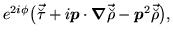
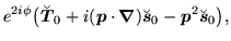
Since all local p-p densities (93) are multiplied under the gauge transformation by phase factors $e^{2i\phi(\mbox{{\boldmath {$r$}}})}$, products of local p-p densities are not gauge invariant. Therefore, all terms not shown explicitly in the p-p energy density [see discussion below Eq. (80)] violate the gauge invariance. On the other hand, products of complex conjugate p-p densities and p-p densities may be gauge invariant. This obviously is the case for the pairing, spin, current, and spin-current p-p densities, while only specific combinations of kinetic, spin-kinetic, and tensor-kinetic densities are gauge invariant.

Complete list of all p-h and p-p gauge-invariant combinations of local densities reads

$\displaystyle G_{k}^{\tau} (\mbox{{\boldmath {$r$}}})$ $\textstyle =$ $\displaystyle \rho _{k}\ofbboxofr\tau _{k}\ofbboxofr - \mbox{{\boldmath {$j$}}} ^{2}_{k}\ofbboxofr ,$ (100)
$\displaystyle G_{k}^{T} (\mbox{{\boldmath {$r$}}})$ $\textstyle =$ $\displaystyle \mbox{{\boldmath {$s$}}} _{k}\ofbboxofr\cdot
\mbox{{\boldmath {$T$}}} _{k}\ofbboxofr - {\mathsf J} ^{2}_{k}\ofbboxofr $  
  $\textstyle =$ $\displaystyle \mbox{{\boldmath {$s$}}} _{k}\ofbboxofr\cdot
\mbox{{\boldmath {$T...
...oldmath {$J$}}} ^{2}_{k}\ofbboxofr - \underline{\mathsf J} ^{2}_{k}\ofbboxofr ,$ (101)
$\displaystyle G_{k}^{\nabla{J}} (\mbox{{\boldmath {$r$}}})$ $\textstyle =$ $\displaystyle \rho _{k}\ofbboxofr\mbox{{\boldmath {$\nabla$}}}\cdot
\mbox{{\bol...
...(\mbox{{\boldmath {$\nabla$}}}\times
\mbox{{\boldmath {$j$}}} _{k}\ofbboxofr ),$ (102)
$\displaystyle G_{k}^{F} (\mbox{{\boldmath {$r$}}})$ $\textstyle =$ $\displaystyle \mbox{{\boldmath {$s$}}}_{k} \ofbboxofr\cdot
\mbox{{\boldmath {$F...
...textstyle{\frac{1}{2}}}\sum_{ab}{\mathsf J}_{kab} {\mathsf J}_{kba} \ofbboxofr $  
  $\textstyle =$ $\displaystyle \mbox{{\boldmath {$s$}}}_{k} \ofbboxofr\cdot
\mbox{{\boldmath {$F...
...\ofbboxofr - {\textstyle{\frac{1}{2}}}\underline{\mathsf J}^{2}_{k}\ofbboxofr ,$ (103)

where $k$=0,1,2,3, and
$\displaystyle \breve{G}_{0}^{T}(\mbox{{\boldmath {$r$}}})$ $\textstyle =$ $\displaystyle \Re\big(\breve{\mbox{{\boldmath {$s$}}}}_0^{\,*}\ofbboxofr\cdot\b...
...0^{\,*}\ofbboxofr\cdot\Delta\breve{\mbox{{\boldmath {$s$}}}}_0 \ofbboxofr\big),$ (104)
$\displaystyle \breve{G}_{0}^{F}(\mbox{{\boldmath {$r$}}})$ $\textstyle =$ $\displaystyle \Re\big(\breve{\mbox{{\boldmath {$s$}}}}_0^{\,*}\ofbboxofr\cdot\b...
...ldmath {$\nabla$}}}\cdot\breve{\mbox{{\boldmath {$s$}}}}_0 \ofbboxofr \vert^2 ,$ (105)
$\displaystyle \breve{G}_{k}^{\tau}(\mbox{{\boldmath {$r$}}})$ $\textstyle =$ $\displaystyle \Re\big(\breve{\rho} _k^{\,*}\ofbboxofr\ \breve{\tau} _k \ofbboxo...
...}}\Re\big(\breve{\rho} _k^{\,*}\ofbboxofr\Delta\breve{\rho} _k \ofbboxofr\big),$ (106)

where $k$=1,2,3. Note that terms of the p-p energy density that depend on $\mbox{{\boldmath {$\nabla$}}}\times\breve{\mbox{{\boldmath {$j$}}}}_0$ and $\mbox{{\boldmath {$\nabla$}}}\cdot\vec{\breve {\mbox{{\boldmath {$J$}}}}}$ are not gauge invariant.

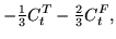
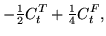
Finally, energy density given by Eqs. (78) and (80) is gauge invariant provided the coupling constants fulfill the following constraints,

$\displaystyle C_{t}^{j}$ $\textstyle =$ $\displaystyle - C_{t}^{\tau} ,$ (107)
$\displaystyle C_{t}^{J0 }$ $\textstyle =$ $\displaystyle - {\textstyle{\frac{1}{3}}} C_{t}^{T} - {\textstyle{\frac{2}{3}}} C_{t}^{F} ,$ (108)
$\displaystyle C_{t}^{J1 }$ $\textstyle =$ $\displaystyle - {\textstyle{\frac{1}{2}}} C_{t}^{T} + {\textstyle{\frac{1}{4}}} C_{t}^{F} ,$ (109)
$\displaystyle C_{t}^{J2 }$ $\textstyle =$ $\displaystyle - C_{t}^{T} - {\textstyle{\frac{1}{2}}} C_{t}^{F} ,$ (110)
$\displaystyle C_{t}^{\nabla j}$ $\textstyle =$ $\displaystyle + C_{t}^{\nabla J} ,$ (111)

for $t$=0,1, and
$\displaystyle \breve{C}_{0}^{\Delta s}$ $\textstyle =$ $\displaystyle - {\textstyle{\frac{1}{4}}} \breve{C}_{0}^{T} ,$ (112)
$\displaystyle \breve{C}_{0}^{\nabla s}$ $\textstyle =$ $\displaystyle + {\textstyle{\frac{1}{4}}} \breve{C}_{0}^{F} ,$ (113)
$\displaystyle \breve{C}_{0}^{\nabla j}$ $\textstyle =$ $\displaystyle \phantom{-} 0 ,$ (114)
$\displaystyle \breve{C}_{1}^{\Delta\rho}$ $\textstyle =$ $\displaystyle - {\textstyle{\frac{1}{4}}} \breve{C}_{1}^{\tau},$ (115)
$\displaystyle \breve{C}_{1}^{\nabla J}$ $\textstyle =$ $\displaystyle \phantom{-} 0 .$ (116)


next up previous
Next: Skyrme interaction energy functional Up: The Energy Density Functional Previous: The Energy Density Functional
Jacek Dobaczewski 2004-01-03