Next: Linear regularization scheme Up: Regularization scheme Previous: Regularization scheme
In this work, all implementations of projection methods are based on the GWT,
which allows for deriving compact and numerically tractable expressions for off-diagonal
matrix elements between Slater determinants. For an arbitrary Slater determinant
![]() ,
by
,
by
![]() we
denote the one that is rotated in space, gauge space, or isospace, for the angular-momentum,
particle-number, or isospin restoration, respectively. Hereafter, we focus our attention
on the AMP, but the presented ideas and methodology can be rather
straightforwardly generalized to the particle-number [5] or isospin projections.
we
denote the one that is rotated in space, gauge space, or isospace, for the angular-momentum,
particle-number, or isospin restoration, respectively. Hereafter, we focus our attention
on the AMP, but the presented ideas and methodology can be rather
straightforwardly generalized to the particle-number [5] or isospin projections.
In order to bring forward the origin of singularities in energy kernels [1,2,3],
it is instructive to recall principal properties
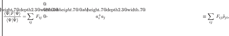
of the standard GWT approach. Let us start with a one-body density-independent operator
![]() . Its off-diagonal kernel (the matrix element
divided by the overlap), can be calculated
with the aid of GWT, and reads [4]:
. Its off-diagonal kernel (the matrix element
divided by the overlap), can be calculated
with the aid of GWT, and reads [4]:
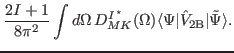
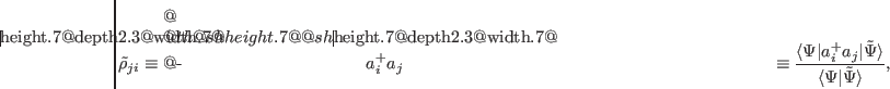
The immediate conclusion stemming from
Eqs. (1)-(2) is that the overlaps, which appear
in the denominators of the matrix element and transition density matrix,
cancel out, and the matrix element
![]() of an arbitrary one-body
density-independent operator
of an arbitrary one-body
density-independent operator ![]() is free from singularities and
can be safely integrated, as in Eq. (3).
is free from singularities and
can be safely integrated, as in Eq. (3).
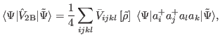
Let us now turn our attention to two-body operators. The most popular two-body effective interactions used in nuclear structure calculations are the zero-range Skyrme [8,9] and finite-range Gogny [10] effective forces. Because of their explicit density dependence, they should be regarded, for consistency reasons, as generators of two-body part of the nuclear EDF. The transition matrix element of the two-body generator reads:
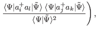
Evaluating the transition matrix element, Eq. (5), with the aid of GWT, one obtains,
 and
and
 vanish, whereas the remaining two contractions give
products of two transition density matrices,
vanish, whereas the remaining two contractions give
products of two transition density matrices,
At variance with the one-body case discussed above, the integrand in
Eq. (10) is inversely proportional to the overlap, thus
containing potentially dangerous (singular) terms. The singularity
disappears only if the sums in the numerator, evaluated at angles
![]() where the overlap
where the overlap
![]() equals
zero, give a vanishing result; such a cancellation requires
evaluating the numerator without any approximations or omitted terms.
An additional singularity is created by the density dependence of the interaction.
equals
zero, give a vanishing result; such a cancellation requires
evaluating the numerator without any approximations or omitted terms.
An additional singularity is created by the density dependence of the interaction.
If some approximation of the numerator is involved, the leading-order singularity goes as:
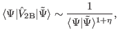 |
(11) |
Thus, the GWT formulation of MR DFT is, in general, singular. In
fact, it is well defined only for
![]() being a true interaction. An example of such an EDF generator is the
density-independent Skyrme interaction SV
being a true interaction. An example of such an EDF generator is the
density-independent Skyrme interaction SV![]() , which is the SV
interaction of Ref. [18] with all the EDF tensor terms
included (these were omitted in the original definition of SV).
Interaction SV
, which is the SV
interaction of Ref. [18] with all the EDF tensor terms
included (these were omitted in the original definition of SV).
Interaction SV![]() was recently used to calculate the
isospin-symmetry-breaking corrections to superallowed
was recently used to calculate the
isospin-symmetry-breaking corrections to superallowed
![]()
![]() -decay by means of the isospin- and angular-momentum
projected DFT formalism [19].
-decay by means of the isospin- and angular-momentum
projected DFT formalism [19].
Progress in development of projection techniques and difficulties in working out reliable regularization schemes for density-dependent interactions [2] increased the demand for density-independent effective interactions and stimulated vivid activity in this field resulting in developing density-independent zero-range [20,21] as well as finite-range [22] forces. The spectroscopic quality of these new forces is, however, still far from satisfactory. In addition, the technology of performing beyond-mean-field calculations with these novel interactions is being developed only now [23,24].
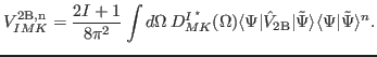
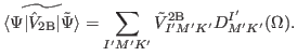
The pathologies arising in the GWT description of the two-body energy kernels come from uncompensated zeros of the overlap matrix. The central idea of this work is to cure the problem by replacing the calculation of projected matrix elements with higher-order quantities, which are regularized by multiplying the integrands with an appropriately chosen power of the overlap:
| (12) |
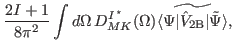
The proposed regularization scheme amounts to
replacing the calculation of matrix elements
![]() , given in Eq. (10), by the calculation of an auxiliary
quantities defined as:
, given in Eq. (10), by the calculation of an auxiliary
quantities defined as:
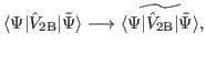
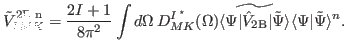
Finally, the regularized matrix elements
 are determined be
requesting that the auxiliary quantities (13), calculated
before and after regularization are equal, that is,
are determined be
requesting that the auxiliary quantities (13), calculated
before and after regularization are equal, that is,
Two variants of such a regularization scheme, dubbed linear
regularization (LR) and quadratic regularization (QR), corresponding
to, respectively, ![]() and
and ![]() , are discussed below in
Secs. 2.2 and 2.3.
, are discussed below in
Secs. 2.2 and 2.3.
Jacek Dobaczewski 2014-12-06

![$\displaystyle \frac{1}{4}\sum_{ijkl} \bar{V}_{ijkl}\left[\tilde{\rho}\right]\;
...
...ineskip}
$\hfil\displaystyle{\hata _l \hata _k}\hfil$\crcr}}}\limits \; \right.$](img34.png)

![$\displaystyle \frac{1}{4}\sum_{ijkl} \bar{V}_{ijkl}\left[\tilde{\rho}\right]\;
...
...tilde{\rho}_{ki}\tilde{\rho}_{lj}
- \tilde{\rho}_{li}\tilde{\rho}_{kj} \right),$](img39.png)
![$\displaystyle \frac{1}{4}\sum_{ijkl} \bar{V}_{ijkl}\left[\tilde{\rho}\right]\;
...
...hata _l\vert\tilde{\Psi}\rangle}{\langle\Psi\vert\tilde{\Psi}\rangle^2}
\right.$](img40.png)
![$\displaystyle \frac{1}{2}\sum_{ijkl} \bar{V}_{ijkl}\left[\tilde{\rho}\right]\;
...
...a ^+_j \hata _l\vert\tilde{\Psi}\rangle}{\langle\Psi\vert\tilde{\Psi}\rangle} .$](img44.png)