


Next: Results
Up: Dependence of single-particle energies
Previous: Introduction
Method
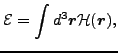
In the present study we consider EDF in the form given
in Refs. [6,7],
 |
(1) |
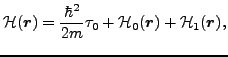
where the energy density
 can be
represented as a sum of the kinetic energy and of the
potential-energy isoscalar (
can be
represented as a sum of the kinetic energy and of the
potential-energy isoscalar ( ) and isovector (
 ) terms,
 |
(2) |
which for the time-reversal and spherical symmetries imposed read:
 |
(3) |
Standard definitions of the local densities  ,
,  , and
, and  were given in Refs. [8,7] and are not repeated here.
Following the parametrization used for the Skyrme forces, we assume
the dependence of the coupling parameters
were given in Refs. [8,7] and are not repeated here.
Following the parametrization used for the Skyrme forces, we assume
the dependence of the coupling parameters
 on the isoscalar density
  as:
as:
 |
(4) |
Similarly as in Ref. [9], we note here that EDF of Eq. (1)
depends linearly on twelve coupling constants,
 and and |
(5) |
for and 1. Therefore, due to the
Hellmann-Feynman theorem [10], derivatives of the
total energy  with respect to the coupling constants
are given by space integrals of densities appearing in Eq. (3)
[9].
with respect to the coupling constants
are given by space integrals of densities appearing in Eq. (3)
[9].
Variation of EDF in Eq. (1) with respect to the Kohn-Sham
orbitals
 , which define the local densities, gives
the standard eigenequation,
, which define the local densities, gives
the standard eigenequation,
 |
(6) |
where the Kohn-Sham one-body Hamiltonian  is obtained as a
functional derivative of EDF with respect to densities, see, e.g.,
Refs.[8,7,11]. It is obvious that also
depends linearly on the coupling constants, and therefore, again due
to the Hellmann-Feynman theorem, derivatives of the s.p. energies
is obtained as a
functional derivative of EDF with respect to densities, see, e.g.,
Refs.[8,7,11]. It is obvious that also
depends linearly on the coupling constants, and therefore, again due
to the Hellmann-Feynman theorem, derivatives of the s.p. energies
 with respect to the coupling constants are also
given by space integrals of densities. As a consequence, we can
expect that these derivatives are generic quantities weakly dependent on a
particular parametrization of the functional, provided the functional
has been adjusted to data and the underlying densities are correct.
with respect to the coupling constants are also
given by space integrals of densities. As a consequence, we can
expect that these derivatives are generic quantities weakly dependent on a
particular parametrization of the functional, provided the functional
has been adjusted to data and the underlying densities are correct.
The aim of the present work is not only to determine these
derivatives but also to estimate to which extent they are generic. Of
course, for a given set of coupling constants, they can be calculated
from the Hellmann-Feynman theorem. Equivalently, their determination
may rely on numerically calculating functions
 ,
where index
,
where index
 is assumed to enumerate the twelve
coupling constants (5). One simple option would be to
calculate them from the finite-difference formula, for example as
is assumed to enumerate the twelve
coupling constants (5). One simple option would be to
calculate them from the finite-difference formula, for example as
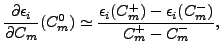 |
(7) |
with values of  and
and  suitably close to
  . Had the
functions
been exactly linear, the Hellmann-Feynman
and finite-difference methods would have given exactly the same
answers. If we aim at determining the degree to which they are not linear
we have to proceed in another way.
. Had the
functions
been exactly linear, the Hellmann-Feynman
and finite-difference methods would have given exactly the same
answers. If we aim at determining the degree to which they are not linear
we have to proceed in another way.
To this end, the method of choice is the linear regression analysis
[12], which makes a hypothesis of linearity and tests it by
determining the regression coefficients and their standard
deviations. In our case, we write the expression
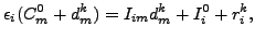 |
(8) |
where
 are the s.p. energies calculated
self-consistently for coupling constants
are the s.p. energies calculated
self-consistently for coupling constants
 that differ from
by suitably small numbers
that differ from
by suitably small numbers  . Index
  enumerates
different choices of these small numbers (which sample the vicinity
of ) and
enumerates
different choices of these small numbers (which sample the vicinity
of ) and  are the residuals between the self-consistent
results and linear approximation given by the regression coefficients
are the residuals between the self-consistent
results and linear approximation given by the regression coefficients
 and
and
 . The regression method minimizes the
residuals by adjusting the regression coefficients and determines
their standard deviations. It is obvious that regression coefficients
constitute estimates of derivatives (7), while
. The regression method minimizes the
residuals by adjusting the regression coefficients and determines
their standard deviations. It is obvious that regression coefficients
constitute estimates of derivatives (7), while
 are very close to
 .
.
The results below were obtained by using
 , where
 to 0.005, depending on the Skyrme functional and nucleus, i.e.,
each of the twelve coupling constants was raised or lowered by the
same percent fraction. (In some cases, for vanishing coupling
constants , appropriate absolute shifts were used.) As a
result, in each case the regression analysis was done by using
to 0.005, depending on the Skyrme functional and nucleus, i.e.,
each of the twelve coupling constants was raised or lowered by the
same percent fraction. (In some cases, for vanishing coupling
constants , appropriate absolute shifts were used.) As a
result, in each case the regression analysis was done by using
 =4096 samples.
Next: Results
Up: Dependence of single-particle energies
Previous: Introduction
Jacek Dobaczewski
2008-05-18