Methods

Estimation of signal's energy density

The two methods discussed below represent the extrema of the wide spectrum of possible time-frequency estimators: spectrogram offers a fast algorithm and well established properties, while MP has the highest presently available resolution at a cost of a high computational complexity. Both these methods offer uniform time-frequency resolution, as opposed to the time-scale approaches (wavelets).

Short time Fourier transform

Short time Fourier transform (STFT or spectrogram) divides the signal into overlapping epochs. Each of these epochs is multiplied by a window function and then subjected to the Fast Fourier Transform [12], providing spectrum with resolution dependent on the epoch's length. We used Hanning windows with overlap 1/2 of its length.

Matching pursuit

Matching pursuit (MP) is an algorithm for a sub-optimal solution of the NP-hard problem of an optimal approximation of a function in a redundant dictionary $D$. It was proposed in [13] for the adaptive time-frequency approximations of signals. In each of the steps the waveform $g_{\gamma_n}$ is matched to the signal $R^n f$, which is the residual left after subtracting results of previous iterations:

$$\left \{ \begin{array}{l} R^0f = f\\ R^nf = <R^nf,g_{\gamma_n}>g_... ... \max_{g_{\gamma_i} \in D } \vert<R^nf, g_{\gamma_i}>\vert \end{array} \right .$$ (1)

where $\arg \max_{g_{\gamma_i} \in D }$ means the $g_{\gamma_i}$ giving the largest value of the product $\vert<R^nf, g_{\gamma_i}>\vert$.

Dictionaries ($D$) for time-frequency analysis of real signals are constructed from real Gabor functions:

$$g_\gamma (t) = K(\gamma)e^{ -\pi\left( \frac{t-u}{s} \right)^2} \sin\left(2 \pi \frac \omega N (t-u)+\phi\right)$$ (2)

$N$ is the size of the signal, $K(\gamma)$ is such that $\vert\vert g_{\gamma}\vert\vert=1$, $\gamma=\{ u, \omega, s, \phi \}$ denotes parameters of the dictionary's functions. For these parameters no particular sampling is a priori defined. In practical implementations we use subsets of the infinite space of possible dictionary's functions. However, any fixed scheme of subsampling this space introduces a statistical bias in the resulting parametrization. In [14] we proposed a solution in terms of MP with stochastic dictionaries, where the parameters of a dictionary's atoms are randomized before each decomposition, or drawn from flat distributions. Results presented in this paper were obtained with such a bias-free implementation.

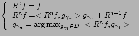
For a complete dictionary the procedure converges to $f$, but in practice we use finite sums:

$$f\approx \sum_{n=0}^M {<R^n f,\; g_{\gamma_n}> g_{\gamma_n} }$$ (3)

From this decomposition we can derive an estimate $E f (t, \omega)$ of the time-frequency energy density of signal $f$, by choosing only auto-terms from the Wigner distribution

$${\mathcal W} f(t, \omega)=\int f \bigl (t + \frac{\tau}{2} \bigr)\; \overline{ f\bigl(t- \frac{\tau}{2} \bigr )\; } e^{- i \omega \tau } d \tau$$ (4)

calculated for the expansion (3). This representation will be a priori free of cross-terms:

$$E f (t, \omega) = \sum_{n=0}^M \vert<R^n f, \;g_{\gamma_n}>\vert^2 \; {\mathcal W} g_{\gamma_n} (t, \omega)$$ (5)

Time-frequency resolution

Time-frequency resolution of signal's representation depends on a multitude of factors, which are even more complicated in the case of the averaged estimates of energy. A general lower bound is given by the uncertainty principle, which states (c.f. [15]) that the product of the time and frequency variances exceeds a constant, which for the frequency defined as inverse of the period (Hz) equals to $\frac 1 {16\pi^2}$:

$$\sigma_t^2\sigma_f^2 \ge \frac 1 {16\pi^2}$$ (6)

It can be proved that equality in this equation is achieved by complex Gabor functions; other functions give higher values of this product. Since the time and frequency spreads are proportional to the square root of the corresponding variances, minimum of their product reaches $\frac 1 {4\pi}$.

However, our attempts to estimate the statistical significance in small resels of area given by (6) resulted in increased "noise", i.e., detections of isolated changes in positions inconsistent across varying other parameters. Therefore we fixed the area of resels at $\frac 1 2$, which at least has certain statistical justification: standard, generally used sampling of the spectrogram gives $\frac 1 2$ as the product of the localization in time (window length less overlap) and in frequency (interval between estimated frequencies). This sampling is based upon statistically optimal properties, namely independent samples for a periodogram of a Gaussian random process (c.f. [16]). Other values of this parameter can be of course considered in practical applications: the software accompanying this paper allows to investigate the impact of changing this parameter.

Integration of MP maps

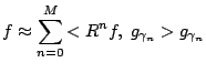
Unlike the spectrogram (STFT, section II-A.1), MP decomposition (section II-A.2) generates a continuous map of the energy density (5). From this decomposition a discrete map must be calculated with a finite resolution. The simplest solution is to sum for each resel the values of all the functions from the expansion (3) in the center of each resel ( $t_i, \omega_i$):

$$E_\textrm{point}(t_i, \omega_i) = \sum_{n} \vert<R^n f, \;g_{\gamma_n}>\vert^2 \; {\mathcal W} g_{\gamma_n} (t_i, \omega_i)$$ (7)

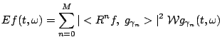
However, for certain structures or relatively large resels, (7) may not be representative for the amount of energy contained in given resel. Therefore we use the exact solution, obtained by integrating for each resel power of all the functions from expansion (3) within the ranges corresponding to the resel's boundaries:

$$E_\textrm{int}(t_i, \omega_i) = \sum_{n} \vert<R^n f, g_{\gamma_n... ...a_i+\frac{\Delta \omega}{2}} {\mathcal W} g_{\gamma_n} (t, \omega) d t d \omega$$ (8)

The difference between (7) and (8) is most significant for structures narrow in time or frequency relative to the dimensions of resels. In this study we used relatively large resel's area and the average difference in energy did not exceed 5-7%.

Statistics

Reference epoch

To quantify changes of the energy density we first define a reference epoch. Properties of the signal in this epoch should reflect the ``normal'' state, i.e. ``stationary'' properties of the signal, in the sense that the measured changes will be relative to these properties.

Strict assumption of stationarity of the signals in the reference epoch would make an elegant derivation of the applied statistics: the repetitions could be then treated as realizations of an ergodic process. Indeed, epochs of EEG up to 10 sec duration (recorded under constant behavioral conditions) are usually considered stationary [17]. However, the assumption of ``constant behavioral conditions'' can be probably challenged in some cases. We cannot test this assumption directly, since the usual length of the reference epoch is too short for a standard test of stationarity. Nevertheless, bootstrapping the available data across the indexes corresponding to time and repetition (number of the trial) simultaneously does not require a strict assumption of ergodicity from the purely statistical point of view. But we must be aware that this fact does not diminish our responsability in the choice of the reference epoch, which in general should be long enough to represent the ``reference'' properties of the signal to which the changes will be related, and at the same time it should be distant enough from the beginning of the recorded epoch (to avoid the influence of border conditions in analysis) and the investigated phenomenon (not to include some event-related properties in the ``reference'').

Permutation test on the difference of means

The values of energy of all the $N$ repetitions in each questioned resel will be compared to energies of resels within the corresponding frequency of the reference epoch. Lets denote the time indexes $t_i$ of resels belonging to the reference epoch as $\{t_i, i \in \textrm{ref}\}$ and their number contained in each frequency slice (defined by the frequency width of a resel) as $\char93 \{\textrm{ref}\}$. We have a total of $N$ repetitions of signals and their time-frequency maps. So for each frequency we have a total of $N\cdot\char93 \{\textrm{ref}\}$ values of energy in the corresponding resels. For each resel at coordinates $\{t_i,\omega_i\}$ we'll compare its energy averaged over $N$ repetitions with the energy averaged over repetitions in resels from the reference epoch in the same frequency. Their difference can be written as:

$$\Delta E_\textrm{int}(t_i, \omega_i)=$$

$$=\frac{1}{N}\sum\limits_{k=1}^N E_\textrm{int}^k(t_i, \omega_i) -... ...\limits_{k=1}^N \sum\limits_{j\in\textrm{ref}} E_\textrm{int}^k(t_j, \omega_i)=$$

$$=\overline{E(t_i,\omega_i)} - \overline{E(t_\textrm{ref},\omega_i)}$$ (9)

where the superscript ``$^k$'' denotes the $k$-th repetition (out of $N$).

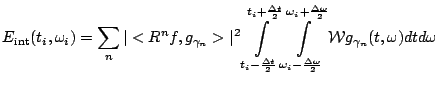
The values of $E_\textrm{int}^k(t_i, \omega_i)$ tend to have (especially for the MP estimates) a highly non-normal distributions. It is caused mainly by the adaptivity and high resolution of the MP approximation. Namely, the areas where no coherent signal's structures are encountered by the algorithm are left completely ``blank", which causes the appearance of peaks around zero in histograms presented in Figure 1. On the contrary, other estimates of energy density provide a more uniform filling of the time-frequency plane, because of lower resolution and cross-terms.

Given these distributions, we cannot justify an application of a parametric test based upon the assumption of normality. In order to preserve high power of the test we estimate the distributions from the data themselves by means of resampling methods (c.f. [19]).

Figure 1: Histograms of powers in the resels from the reference epoch of the analyzed signals (Dataset II) for two frequencies: 12 Hz (a, c and e) and 30 Hz (b, d and f). First four plots (a-d) are for the MP estimates: distribution is highly skewed toward the zero power, especially in cases when less waveforms are used for the representation (a and b). Lower panels (e and f) present histograms of powers estimated by STFT for the same frequency slices. Vertical scales (number of cases) differ, horizontal (energy) are kept constant across the subplots.

We are testing the null hypothesis of no difference in means between the values $\{E_\textrm{int}^k(t_i, \omega_i), k\in 1\dots N\}$ of the $i$-th resel and all those in corresponding reference region $\{E_\textrm{int}^k(t_j, \omega_i), k\in 1\dots N, j\in\textrm{ref}\}$, that is energy values for the same frequency band for the resels falling into the reference epochs in all the repetitions (trials). A straightforward application of the idea of the permutation tests for each resel consists of:

1. mixing the values of $E_\textrm{int}$ for all the repetitions of the resel under investigation and all the resels of the corresponding reference epoch,
2. drawing from this ensemble (without replacement) one of the $\binom{N\cdot(\char93 \{\textrm{ref}\}+1)}{N}$ possible combinations (i.e. permutations not distinguishing different ordering), subdividing it into two sets containing $N$ and $N\cdot\char93 \{\textrm{ref}\}$ elements
3. calculating for the above sets the difference of means (9)
4. repeating the two above steps $N_\textrm{rep}$ times and estimating from the obtained values distribution of the statistics (9) under the null hypothesis
5. based upon this distribution, calculating the $p$ value for the actual difference of means

The number of permutations giving values of (9) exceeding the observed value has a binomial distribution for $N_\textrm{rep}$ repetitions with probability $\alpha$. Its variance equals $N_\textrm{rep}\alpha(1-\alpha)$. The relative error of $\alpha$ will be then (c.f. [19])

$$\frac{\sigma_\alpha}{\alpha}=\sqrt{\frac{(1-\alpha)}{\alpha N_\textrm{rep}}}$$ (10)

To keep this relative error at 10% for a significance level $\alpha$=5%, $N_\textrm{rep}=2000$ is enough. Unfortunately, due to the problem of multiple comparisons discussed in Section II-D.5, we need to work with much smaller values of $\alpha$. In this study $N_\textrm{rep}$ was set to $2\cdot10^5$ or $2\cdot10^6$, which resulted in large computation times. Therefore we implemented also a less computationally demanding approach, described in the following section.

Bootstrap with pseudo-$t$ statistics

For a large number of points in each frequency of the reference region $\char93 \{\textrm{ref}\}$, the statistics estimated in the previous section is dominated mainly by the values from the reference region, with little influence from the current resel. Estimation of its distribution only from the resels in the reference region would save a lot of computations. However, we still want to account for the different variances of $E_\textrm{int}^k$ revealing the variability of the $N$ repetitions. Therefore we replace the simple difference of means by the pseudo-$t$ statistics:

$$t=\frac{\Delta E_\textrm{int}(t_i, \omega_i)}{s_{\Delta}}$$ (11)

Where $\Delta E_\textrm{int}$ is defined as in Eq. (9), and $s_\Delta$ is the pooled variance of the reference epoch and the investigated resel. We estimate the distribution of this magnitude from the data in the reference epoch (for each frequency $N\cdot\char93 \{\textrm{ref}\}$ values) by drawing with replacement two samples of sizes $N$ and $N\cdot\char93 \{\textrm{ref}\}$ and calculating for each such replication statistics (11). This distribution is approximated once for each frequency. Then for each resel the actual value of (11) is compared to this distribution yielding $p$ for the null hypothesis.

Computational complexity

Both presented above methods are computer-intensive, which nowadays causes no problems in standard applications. However, corrections for multiple comparisons imply much lower effective values of cutoff probabilities $p_k$ (see the next section II-D.5). For the analysis presented in this study both the FDR (False Discovery Rate, see next section) and Bonferroni-Holmes adjustments gave critical values of the order of $5\cdot 10^{-5}$ for the Dataset II (larger number of investigated resels, see section II-E ``Experimental Data'') and $5\cdot 10^{-4}$ for Dataset I. If we set this for $\alpha$ in eq. (10), we obtain minimum of $N_\textrm{rep}=2\cdot 10^6$ or $2\cdot10^5$ bootstrap or resampling repetitions to achieve 10% relative error for $\alpha$.

Comparisons on presented datasets confirmed very similar results for both these procedures, as expected from the discussion in section II-D.3. This served as a justification to use in practice the pseudo-$t$ bootstrapping, which is significantly faster.

Adjustment for multiplicity

In the preceding two sections we estimated the achieved significance levels $p$ for a null hypotheses of no change of the average energy in a single resel compared to the reference region in the same frequency. Statistics of these tests for different resels are not independent--neither in the time nor in the frequency dimension, and the structure of their correlation is hard to guess a priori.

Adjusting results for multiplicity is a very important issue in case of such a large amount of potentially correlated tests. We chose for this step the procedure assessing the False Discovery Rate (FDR, proposed in [20]). Unlike the adjustments for the family-wise error rate (FWE), it controls the ratio $q$ of the number of the true null hypotheses rejected to all the rejected hypotheses. In our case this is the ratio of the number of resels to which significant changes are wrongly attributed to the total number of resels revealing changes.

The main result presented in [20] requires the test statistics to have positive regression dependency on each of the test statistics corresponding to the true null hypothesis. We use a slightly more conservative version, which controls FDR for all other forms of dependency. Let's denote the total number of performed tests, equal to the number of questioned resels, as $m$. If for $m_0$ of them the null hypothesis of no change is true, [20] proves that the following procedure controls the FDR at the level $q\frac{m_0}{m}\le q$:

1. Order the achieved significance levels $p_i$, approximated in the previous section for all the resels separately, in an ascending series: $p_1\le p_2\le \dots \le p_m$
2. Find

   $$k=\max\{i: p_i \le \frac{i}{m\sum_{j=1}^{m}\frac{1}{j}} q\}$$ (12)

   
   

3. Reject all hypotheses for which $p\le p_k$

Another, more conservative correction for multiplicity is the step-down Bonferroni-Holmes adjustment [11]. It relies on comparing the $p_i$ values, ordered as in point (1.) above, to $\dfrac{\alpha}{m-i+1}$, where $\alpha$ controls the family-wise error. We used $\alpha = q = 0.05$, which for the FDR relates to the possibility of erroneous detection of changes in one out of 20 resels indicated as significant.

According to the comparisons performed on the two discussed datasets, false discovery rate (FDR) resulted--as expected--to be less conservative that the stepdown Bonferroni-Holmes procedure. It has also a more appealing interpretation than the family-wise error (FWE) of Bonferroni-like procedures. Both these procedures take negligible amounts of computations.

Experimental data

We present results for two datasets: what we shall refer as the "Dataset I" comes from another study, described in [10]. Dataset II was collected especially for the purpose of this study. The main reason of this was the need for longer than usual epochs of EEG between the stimuli repetitions to confirm the absence of false positives detections in neutral time epochs.

Dataset I

Twenty-year old right-handed subject was lying in a dim room with open eyes. Movements of index finger were performed approximately 5 seconds after a quiet sound generated every 10 to 14 seconds and detected by a micro-switch. The experiment was divided into 5 minutes long alternating sessions for right and left index finger movements, with 3 minutes breaks in between.

EEG was registered from electrodes placed at positions selected from the extended 10-20 system, sampled at 256 Hz, analog bandpass filtered in the 0.5-100 Hz range and sub-sampled offline to 128 Hz. For data processing, EEG was divided into 8 seconds long epochs, with movement onset in the 5th second. We present analysis of 57 artifact-free trials of right hand finger movement from the electrode C1 referenced to Cp1, Fc1, Cz and C3 (local average reference).

Dataset II

Thirty one-year old right-handed subject was half lying in a dim room with open eyes. Movement of the thumb, detected by a micro-switch, were performed approximately 5 seconds (at a subject's choice) after a quiet sound generated approximately every 20 seconds. Experiment was divided into 15-minutes sessions, and recorded EEG into 20-sec long epochs with the movement occurring in the 12th second. After artifacts rejection, 124 epochs were left for the analysis presented hereby.

EEG was registered from electrodes at positions selected from the 10-20 system. For the analysis we choose the C4 electrode (contra-lateral to the hand performing movements) in the local average reference. Analog filters were 100-Hz low-pass and 50-Hz notch. Signal was sampled at 250 Hz and down-sampled offline to 125 Hz.