


Next: Infinite Nuclear Matter
Up: Gamow-Teller strength and the
Previous: Local Densities and Currents
Energy density functional from the two-body Skyrme force
The standard two-body Skyrme force is given by [2,33]
where
 )
is the spin-exchange operator,
)
is the spin-exchange operator,
 acts to the right, and
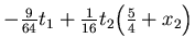
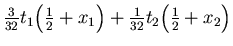
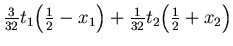
 acts to the left. Calculating the Hartree-Fock expectation value from
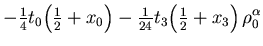
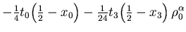
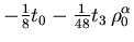
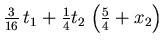
this force yields the energy functional given in Eq. (12) with the coupling constants:
acts to the left. Calculating the Hartree-Fock expectation value from
this force yields the energy functional given in Eq. (12) with the coupling constants:
 |
= |
 |
|
 |
= |
 |
|
| C0s |
= |
 |
|
| C1s |
= |
 |
|
 |
= |
 |
|
 |
= |
 |
|
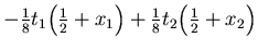
| C0T |
= |
![$\displaystyle \eta_J \,
\Big[
- {\textstyle\frac{{1}}{{8}}} t_1 \Big( {\textsty...
...xtstyle\frac{{1}}{{8}}} t_2 \Big( {\textstyle\frac{{1}}{{2}}} + x_2 \Big)
\Big]$](img206.png) |
|
| C1T |
= |
![$\displaystyle \eta_J \,
\Big[ - {\textstyle\frac{{1}}{{16}}} t_1
+ {\textstyle\frac{{1}}{{16}}} t_2
\Big]$](img207.png) |
|
 |
= |
 |
|
 |
= |
 |
|
 |
= |
 |
|
 |
= |
 |
|
 |
= |
 |
|
 |
= |
 |
|
 |
= |
0 |
|
 |
= |
0 , |
(33) |
nine of which are independent. Although in this approach
 ,
many parameterizations of the Skyrme
interaction set
,
many parameterizations of the Skyrme
interaction set  .
That violates the interpretation
of the Skyrme functional as an expectation value of a real two-body
interaction and removes the rationale for calculating the time-odd
coupling constants from (34). For Skyrme interactions with a
generalized spin-orbit interaction [42], e.g. for SkI3,
SkI4, SkO, or SkO', the spin-orbit coupling constants are given by
.
That violates the interpretation
of the Skyrme functional as an expectation value of a real two-body
interaction and removes the rationale for calculating the time-odd
coupling constants from (34). For Skyrme interactions with a
generalized spin-orbit interaction [42], e.g. for SkI3,
SkI4, SkO, or SkO', the spin-orbit coupling constants are given by
 |
(34) |
The resulting terms in the energy functional again cannot be represented
as the HF expectation value of a two-body spin-orbit potential (see,
e.g., [41]), again violating the assumptions behind the
calculation of the time-odd coupling constants in (34).
As Eqs. (34) represent the standard approach to the time-odd
coupling constants, it is worthwhile to take a look at the actual
values. Table 4 compares them for several Skyrme
forces. None of these parameterizations was obtained from observables
sensitive to the time-odd terms in the energy functional. Differences
among the forces merely reflect various strategies for adjusting the
time-even coupling constants. Values of the density-dependent isoscalar
coupling constants C0s, either at
 or at
or at
 ,
are scattered
in a wide range. This is probably one of the main sources of
differences in the predictions of the forces for time-odd corrections
to rotational bands. For the SLyx forces, C0s [0]
is negative, which is unusual; most often
this part of the isoscalar spin-spin interaction is repulsive at all
densities. The difference will probably cause visible differences
in rotational properties whenever the spin density is large at the
surface. All the forces agree on the isovector coupling constant
C1s, especially at the saturation density, i.e.,
,
are scattered
in a wide range. This is probably one of the main sources of
differences in the predictions of the forces for time-odd corrections
to rotational bands. For the SLyx forces, C0s [0]
is negative, which is unusual; most often
this part of the isoscalar spin-spin interaction is repulsive at all
densities. The difference will probably cause visible differences
in rotational properties whenever the spin density is large at the
surface. All the forces agree on the isovector coupling constant
C1s, especially at the saturation density, i.e.,
![$C_1^s[\rho_{\rm nm}] \approx 100 \;$](img226.png) MeV fm3. This
simply follows from the fact that, assuming Eq. (34),
C1s is proportional to the time-even
MeV fm3. This
simply follows from the fact that, assuming Eq. (34),
C1s is proportional to the time-even  that is
fixed from binding energies and radii.
that is
fixed from binding energies and radii.
Next: Infinite Nuclear Matter
Up: Gamow-Teller strength and the
Previous: Local Densities and Currents
Jacek Dobaczewski
2002-03-15