The HFB equations

Minimization of the energy functional of Eq. (72) with respect to the p-h and p-p density matrices, which fulfill Eqs. (13) under auxiliary conditions

$$\int {{\rm d}}^3\mbox{{\boldmath {$r$}}}\rho_n(\mbox{{\boldmath {$r$}}}) = N,$$ (196)

$$\int {{\rm d}}^3\mbox{{\boldmath {$r$}}}\rho_p(\mbox{{\boldmath {$r$}}}) = Z,$$ (197)

leads to the HFB equation of the form:

$$\left[\hat{\breve{\mathcal H}},\hat{\breve{\mathcal R}}\right] =0.$$ (198)

The generalized density matrix $\hat{\breve{\mathcal R}}$ is given by Eq. (16) and the generalized mean-field Hamiltonian is defined as

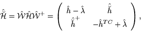$$\hat{\breve{\mathcal H}} = \hat{\mathcal W}\hat{\mathcal H}\... ...reve{h}}^{+} & -\hat{h}^{TC}+\hat{\lambda}\end{array}\right) ,$$ (199)

with the Lagrange multiplier given by

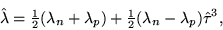$$\hat{\lambda}={\textstyle{\frac{1}{2}}}(\lambda_n+\lambda_p)+{\textstyle{\frac{1}{2}}}(\lambda_n-\lambda_p)\hat{\tau}^3,$$ (200)

where $\lambda_n$ and $\lambda_p$ are the neutron and proton Fermi levels, respectively.

The usual method of solving the HFB equation (199) is to solve in a self-consistent way the eigenvalue problem,

$$\hat{\breve{\mathcal H}}(x',x)\bullet \Phi (x;E) = E\Phi (x';E),$$ (201)

for the generalized mean-field Hamiltonian, and then to construct the generalized density matrix,

$$\hat{\breve{\mathcal R}}(x,x')= \sum_{E\in {\mathcal E}}\Phi(x;E)\Phi^+(x';E),$$ (202)

as a projection operator onto the set of the quasihole (occupied) states $\Phi$ belonging to a subset of energy spectrum, $\mathcal E$. For a local mean-field Hamiltonian, Eq. (202) is a system of eight second-order differential equations, in general with complex coefficients. Usual four dimensions corresponding to upper and lower HFB components and to two spin projections are here multiplied by another factor of two due to the isospin projections. Altogether, Eq. (202) corresponds to a system of sixteen equations within the domain of real numbers. When specific symmetry conditions are imposed on solutions, this number can be reduced in a standard way, see Ref. [184] for the analysis pertaining to spherical symmetry.

The energy spectrum of generalized mean-field Hamiltonian has been discussed in Ref. [5]. The only difference with the present case is that here the eigenvalue problems for neutrons and protons in Eq. (202) cannot be separated. It is well known, that the eigenvalues of $\hat{\breve{\mathcal H}}$ appear in pairs of opposite signs. For each quasihole state of energy $E$

$$\Phi (\mbox{{\boldmath {$r$}}}st;E)=\left(\begin{array}{c}\v... ...st;E)\\ \psi (\mbox{{\boldmath {$r$}}}st;E)\end{array}\right)$$ (203)

there exists a quasiparticle state

$$\Phi (\mbox{{\boldmath {$r$}}}st;-E)=4st\left(\begin{array}{... ...}(\mbox{{\boldmath {$r$}}}\,\mbox{$-s-t$};E)\end{array}\right)$$ (204)

belonging to energy $-E$. In the case of absence of external fields, bound states (when $\varphi$ and $\psi$ are both localized) exist only when both Fermi levels, $\lambda_n$ and $\lambda_p$, are negative. Discrete quasihole energy levels lie within the range ${\mathcal L}<E<-{\mathcal L}$, where ${\mathcal L}=\max (\lambda_n,\lambda_p)<0$. The ground-state solution corresponds to occupying states having negative energies; then the set ${\mathcal E}$ consists of a number of discrete levels lying inside segment $({\mathcal L},0)$ and the continuous spectrum with $-\infty<E<{\mathcal L}$.

Traditionally, one solves Eq. (202) for the quasiparticle states of positive energies rather than for the negative ones. Then, the discrete spectrum is within the segment $0<E<-{\mathcal L}$ and energies $E>-{\mathcal L}$ belong to the continuum. Having found the wavefunctions $\Phi (\mbox{{\boldmath {$r$}}}st;E)$ for $E>0$ one uses Eq. (205) to construct the density matrix, i.e.,

$$\hat{\breve{\mathcal R}}(x,x')= \sum_{E>0}\Phi(x;-E)\Phi^+(x';-E).$$ (205)

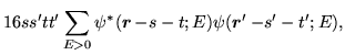
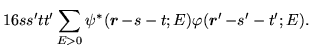
The p-h and p-p density matrices are then expressed as

$$\hat{\rho}(\mbox{{\boldmath {$r$}}}st,\mbox{{\boldmath {$r$}}}'s't') = 16ss'tt'\sum_{E>0}\psi^{\ast}(\mbox{{\boldmath {$r$}}}\,\mbox{$-s-t$};E)\psi (\mbox{{\boldmath {$r$}}}'\,\mbox{$-s$}'-t';E),$$ (206)

$$\hat{\breve{\rho}}(\mbox{{\boldmath {$r$}}}st,\mbox{{\boldmath {$r$}}}'s't') = 16ss'tt'\sum_{E>0}\psi^{\ast}(\mbox{{\boldmath {$r$}}}\,\mbox{$-s$}-t;E)\varphi (\mbox{{\boldmath {$r$}}}'\,\mbox{$-s$}'-t';E).$$ (207)