Next: The HFB equations
Up: Local Density Approximation for
Previous: The p-p channel
The P-H and P-P Mean Fields
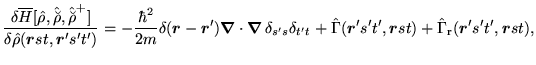
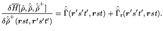
By varying the energy functional (72) with respect to the
density matrices one obtains the p-h and p-p mean
field Hamiltonians,
The rearrangement potentials
 and
and
 result from the density
dependence of effective interactions on the p-h and
p-p densities, respectively. Usually effective interactions
are assumed to depend only on the p-h density matrix (most
often, only on the isoscalar particle density
result from the density
dependence of effective interactions on the p-h and
p-p densities, respectively. Usually effective interactions
are assumed to depend only on the p-h density matrix (most
often, only on the isoscalar particle density  ). In that case
the p-p rearrangement potential vanishes. However, one cannot
forget that the dependence of the p-p interaction on the particle
density results in a corresponding contribution to the p-h
rearrangement potential. In what follows, to simplify the
presentation we do not show the rearrangement terms explicitly.
). In that case
the p-p rearrangement potential vanishes. However, one cannot
forget that the dependence of the p-p interaction on the particle
density results in a corresponding contribution to the p-h
rearrangement potential. In what follows, to simplify the
presentation we do not show the rearrangement terms explicitly.
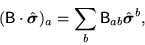
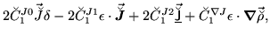
Within the LDA, the mean-field Hamiltonians being originally, like the Skyrme interaction
of Eq. (117), either distributions or derivatives of distributions, can,
when acting as the integral kernels, be expressed as local, momentum
dependent operators, i.e.,
The kinetic energy term in Eq. (158) is already expressed in such a form.
The mean-fields Hamiltonians
are the second-order operators in momentum
and matrices in the spin and isospin spaces. The
isospin structure of the local p-h and p-p mean-field Hamiltonians
reads
respectively.
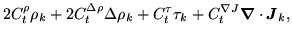
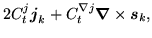
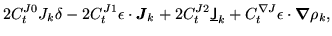
The isoscalar and isovector parts of the p-h mean-field Hamiltonian
can be presented in the compact form
for  , and where
 |
(165) |
for  , is the
  'th component of a space vector. The names
of symbols are inspired by those introduced in Ref. [172].
Since the p-h density matrix is hermitian, the p-h
mean-field Hamiltonian is also hermitian and, thus, all the
potentials,
'th component of a space vector. The names
of symbols are inspired by those introduced in Ref. [172].
Since the p-h density matrix is hermitian, the p-h
mean-field Hamiltonian is also hermitian and, thus, all the
potentials,  ,
,  ,
,  ,
,
 ,
,
 ,
,
 , and
, and
 are real.
The general form of the mean-field Hamiltonian (164) can be
constructed from the momentum
 and spin
 operators, based only on the symmetry
properties. Apart from the one-body kinetic energy [the first term in
Eq. (164)], the expansion in momentum gives: (i) zero-order
terms with scalar () and pseudovector (
)
potentials, (ii) first-order terms with vector (
) and
pseudotensor () potentials, (iii) second-order-scalar
terms with scalar () and pseudoscalar (
) effective
masses, and (iv) second-order-tensor terms. In principle, the most
general form of the last category should involve tensor and
third-order-pseudotensor potentials. However, in Eq. (164) we
show only the particular form of it that corresponds to the energy
density (78).
operators, based only on the symmetry
properties. Apart from the one-body kinetic energy [the first term in
Eq. (164)], the expansion in momentum gives: (i) zero-order
terms with scalar () and pseudovector (
)
potentials, (ii) first-order terms with vector (
) and
pseudotensor () potentials, (iii) second-order-scalar
terms with scalar () and pseudoscalar (
) effective
masses, and (iv) second-order-tensor terms. In principle, the most
general form of the last category should involve tensor and
third-order-pseudotensor potentials. However, in Eq. (164) we
show only the particular form of it that corresponds to the energy
density (78).
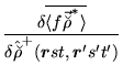
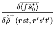
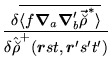
According to Eqs. (158) the p-h mean-field Hamiltonian is the functional derivative
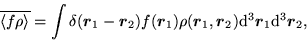
of the energy functional over the hermitian p-h density matrix. Functional derivatives of integrals
of type:
 |
(166) |
where function  is treated as independent of densities and
  represents a p-h non-local density,
can easily be calculated using Eqs. (20) and (24). Bearing in mind that
represents a p-h non-local density,
can easily be calculated using Eqs. (20) and (24). Bearing in mind that
one has
for . The functional derivatives of integrals of local differential densities are obtained from
Eqs. (168) through integration by parts. Then, the functional derivatives become dependent
on derivatives of the Dirac delta function and thus, in accordance with Eqs. (160), again act as local
differential operators.
They read:
for and  .
Calculations
of the functional derivatives over the density matrix are equivalent
to the rules for variations over single-particle wavefunctions given
by Engel et al. [172].
Using formulae given above, Eqs. (168)-(172),
one obtains the following relations between the
potentials defining the p-h mean field (164) and the
local p-h densities defining the energy density (78),
.
Calculations
of the functional derivatives over the density matrix are equivalent
to the rules for variations over single-particle wavefunctions given
by Engel et al. [172].
Using formulae given above, Eqs. (168)-(172),
one obtains the following relations between the
potentials defining the p-h mean field (164) and the
local p-h densities defining the energy density (78),
 |
 |
 |
(173) |
 |
|
 |
(174) |
 |
|
 |
(175) |
 |
|
 |
(176) |
 |
|
 |
(177) |
 |
|
 |
(178) |
 |
|
 |
(179) |
for .
All coupling constants  in Eqs. (174) are taken with
 =0 for
  (isoscalars), and with =1 for
  1,2,3
(isovectors). Symbol
1,2,3
(isovectors). Symbol  is the unit space tensor, and
 stands for the antisymmetric space tensor
with components:
stands for the antisymmetric space tensor
with components:
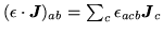 , so that, according to Eq. (165), its action on a vector is obviously the vector
product:
, so that, according to Eq. (165), its action on a vector is obviously the vector
product:
 .
.
The p-p mean-field Hamiltonian has the following
isoscalar and isovector components:
Contrary to the p-h Hamiltonian (164), the p-p
Hamiltonian (181) can be non-hermitian, because potentials
 ,
,
 ,
,
 ,
,
 ,
,
 ,
,
 , and
, and
 are, in general, complex quantities. This
is so, because the p-p density matrix is, in general, not
hermitian. Therefore, the energy functional should be treated as a
functional of both
are, in general, complex quantities. This
is so, because the p-p density matrix is, in general, not
hermitian. Therefore, the energy functional should be treated as a
functional of both
 and
and
 .
.
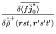
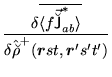
The p-p mean-field Hamiltonian is the functional derivative of
the energy functional over
, whereas the
hermitian conjugate Hamiltonian is the functional derivative over
. The p-p densities are, according to
Eqs. (22) and (26), functions of
, while the complex conjugate densities are
functions of
.
When calculating the p-p functional derivatives, one cannot
forget that the p-p density matrix fulfills symmetry condition
(12), implying that the p-p densities are either
symmetric or antisymmetric functions, Eqs. (34).
Therefore, the calculation of functional derivatives over either
or
is similar to that
leading to Eqs. (168)-(172), however,
instead of Eq. (167) one has:
 |
(182) |
In the expressions for functional derivatives, this gives either
cancellation or addition of terms coming from the two components of
the right-hand side of Eq. (183). Finally, the
non-vanishing derivatives are
for .
Using Eqs. (184)-(186) one obtains the
following relations between the potentials defining the p-p
mean-field Hamiltonian (181) and the local p-p
densities defining the energy density (80):
 |
|
 |
(189) |
 |
|
 |
(190) |
 |
|
 |
(191) |
 |
|
 |
(192) |
 |
|
 |
(193) |
 |
|
 |
(194) |
 |
|
 |
(195) |
In the case of the zero-range pairing force (151), the isovector p-p
potential is proportional to the p-p isovector density while the isoscalar
field has a very different structure, i.e., it
is proportional to the scalar product of spin
and the p-p spin density
 . This immediately suggests
that there exists a connection between the isoscalar pairing
and the p-p spin saturation, which is influenced by the spin-orbit splitting.
In this context, let us remind the shell-model study [20] which discusses
the relation between the magnitude of the
. This immediately suggests
that there exists a connection between the isoscalar pairing
and the p-p spin saturation, which is influenced by the spin-orbit splitting.
In this context, let us remind the shell-model study [20] which discusses
the relation between the magnitude of the  =0 pairing and the
spin-orbit splitting.
=0 pairing and the
spin-orbit splitting.
Next: The HFB equations
Up: Local Density Approximation for
Previous: The p-p channel
Jacek Dobaczewski
2004-01-03
![$\displaystyle - \frac{\hbar^{2}}{2m}\mbox{{\boldmath {$\nabla$}}}^2\delta_{s's}...
...
+ ({\mathsf B}_k\ofbboxofr\cdot\hat{\mbox{{\boldmath {$\sigma$}}}}_{s's})\big]$](img509.png)