


Next: Time-frequency energy distribution
Up: The method
Previous: Matching Pursuit algorithm
Discrete dyadic Gabor dictionary
A waveform (atom) from a time-frequency dictionary can be expressed as
translation ( ), dilation (
 ) and modulation (
 ) of a
window function
) of a
window function

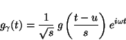 |
(7) |
Optimal time-frequency resolution is obtained for gaussian  ,
which for the analysis of real-valued discrete signals gives a dictionary of
Gabor functions (sine-modulated gaussians):
,
which for the analysis of real-valued discrete signals gives a dictionary of
Gabor functions (sine-modulated gaussians):
 |
(8) |
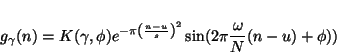
The value of
 is such that
 .
Complete sampling of discrete parameters
.
Complete sampling of discrete parameters
 , where
  is the signal's size in points, produces a
huge dictionary even for relatively small .
Therefore in the "classical" implementation proposed by Mallat and
Zhang [Mallat and Zhang, 1993] dictionary's atoms parameters are chosen from
dyadic sequences. For a discrete signal of length
is the signal's size in points, produces a
huge dictionary even for relatively small .
Therefore in the "classical" implementation proposed by Mallat and
Zhang [Mallat and Zhang, 1993] dictionary's atoms parameters are chosen from
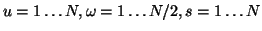
dyadic sequences. For a discrete signal of length  sampling is
governed by a new parameter--octave
sampling is
governed by a new parameter--octave  (integer). Scale ,
corresponding to atom's width in time, is chosen from dyadic sequence
(integer). Scale ,
corresponding to atom's width in time, is chosen from dyadic sequence
 . Parameters and , corresponding
to atom's position in time and frequency, respectively, are sampled
for each octave with an interval
. Parameters and , corresponding
to atom's position in time and frequency, respectively, are sampled
for each octave with an interval  .
.
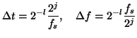
Size of this dictionary (and the resolution of decomposition) can be
increased by oversampling by  (
( ) the time and frequency
parameters and . Resulting dictionary has
) the time and frequency
parameters and . Resulting dictionary has
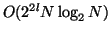 waveforms, so the computational complexity increases with
oversampling by . Time and frequency resolutions increase by the
same factor:
waveforms, so the computational complexity increases with
oversampling by . Time and frequency resolutions increase by the
same factor:
 |
|
|
(9) |
where  is the sampling frequency of analyzed signal. Resolution is
hereby understood as the distance between centers of dictionary's
atoms neighboring in time or frequency, and depends on the octave
(scale ). Scale in turn corresponds to the width of an
atom in time (and frequency). We can define a time width of a
time-frequency atom as a half-width of the window function :
is the sampling frequency of analyzed signal. Resolution is
hereby understood as the distance between centers of dictionary's
atoms neighboring in time or frequency, and depends on the octave
(scale ). Scale in turn corresponds to the width of an
atom in time (and frequency). We can define a time width of a
time-frequency atom as a half-width of the window function :
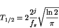 |
(10) |
In spite of the oversampling, the algorithm still looks for signal's
expansion only over a relatively small subset of the possible
dictionary's functions. Issues related to the particular structure of
this subset will be discussed in the section ``Stochastic dictionaries''.
Next: Time-frequency energy distribution
Up: The method
Previous: Matching Pursuit algorithm
Piotr J. Durka
2001-06-11