From equation (6) we can derive a time-frequency
distribution of signal's energy by adding Wigner distributions of
selected atoms [Mallat and Zhang, 1993]. Calculating the Wigner distribution
directly from equations (2) and
(6) would yield
The double sum, containing cross Wigner distributions of different
atoms from the expansion given in eq. (6),
corresponds to the cross terms generally present in Wigner
distribution. These terms one usually tries to remove in order to
obtain a clear picture of the energy distribution in the
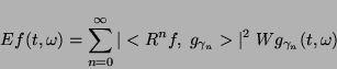
time-frequency plane. Removing these terms from eq. (11) is
straightforward--we keep only the first sum; we can define a
magnitude
![]() :
:
Wigner distribution of a single time-frequency atom ![]() satisfies
satisfies
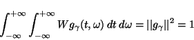 |
(13) |
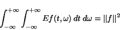 |
(14) |
![\begin{displaymath}
\begin{array}{ll}
W f = & \sum_{n=0}^\infty \vert<R^n f, \;g...
... f, \; g_{\gamma_m}>} W[g_{\gamma_n}, g_{\gamma_m}]
\end{array}\end{displaymath}](img48.png)