We analyze the situation by supposing that the GT energies and strengths
are linear functions of four coupling constants, i.e.,
The sample of QRPA calculations covers
the physically interesting range of values for the coupling constants.
We present here results from a sample defined by the hypercube
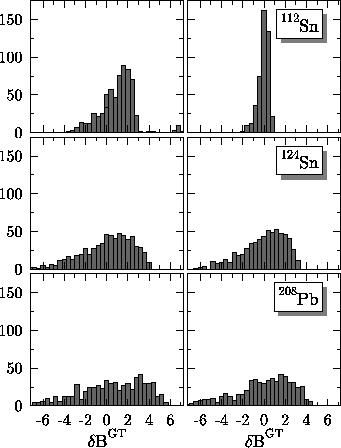
The left panels in Figs. 11 and 12
contain histograms of deviations
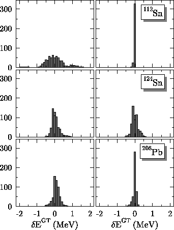 |
As can be seen from Figs. 6, 8, 9, and 10, the dependence of both the resonance energy and the strength in the resonance on the coupling constants is not linear for the entire region of coupling constants. Although our sample is restricted to the area around the reasonable values, at times we leave the region where the regression can safely be performed. Furthermore, for certain combinations of the coupling constants (especially at a weak coupling), there are competing states that carry strength similar to that of the GT ``resonance.'' (These states often merge into the resonance at a larger coupling.) Finally, the resonance can be fragmented into many (sometimes up to 15) states. Therefore, we remove certain areas of parameter space where the determination of either the energy or the strength of the GT resonance is ambiguous. Such areas are almost always singled out by particularly large deviations from the fitted values.
After reducing the sample in this way, we obtain the histograms in the
right panels of Figs. 11
and 12. These illustrate the quality of the
regression fits obtained for samples of N=542, 664,
and 618 in 112Sn, 124Sn, and 208Pb, respectively.
Tables 2 and 3 list
the corresponding values of the regression coefficients, as
well as the standard deviations for the GT energies
and strengths within each of the samples.
|
|
Figures 11 and 12 and the standard
deviations obtained in the reduced and full samples (Tables
2 and 3) show that the description
obtained by removing a small number of points beyond the region of
linearity is quite good. The GT resonance energies are now reproduced
within about ![]() 200keV or less. The description of the resonant GT
strengths is also improved, especially in 112Sn, although here the
linear regression cannot work too well because the strengths saturate at
strong coupling. Nevertheless, the coefficients listed in Tables
2 and 3 allow a fairly reliable estimate of
the QRPA values for any combination of the coupling constants. The
values of the coefficients in Tables 2 and 3
show that
200keV or less. The description of the resonant GT
strengths is also improved, especially in 112Sn, although here the
linear regression cannot work too well because the strengths saturate at
strong coupling. Nevertheless, the coefficients listed in Tables
2 and 3 allow a fairly reliable estimate of
the QRPA values for any combination of the coupling constants. The
values of the coefficients in Tables 2 and 3
show that
![]() and
and
![]() strongly
influence properties of the GT resonance, and that both the energies and
the resonant strengths increase when these coupling constants increase.
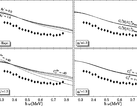
CT1 has a weaker effect in the opposite direction, while Cs1[0]
is less important still.
strongly
influence properties of the GT resonance, and that both the energies and
the resonant strengths increase when these coupling constants increase.
CT1 has a weaker effect in the opposite direction, while Cs1[0]
is less important still.
Without presenting detailed results, we report here on two other attempts at regression analysis. We tried to analyze the results for all the three nuclei, 112Sn, 124Sn, and 208Pb, simultaneously by adding terms e5(N-Z) and b5(N-Z) to the regression formulas (4.4). Linear scaling might be obtained by analyzing the QRPA results for very many nuclei, where the effects due to shell structure could average out. In our small sample, shell structure is obviously important. We also tried the regression analysis with CT1 = -9.172MeVfm5 fixed at its SkO' value (see Table 4), and without the terms e4 and b4 in the regression formulae (4.4), so that the functional's gauge invariance was preserved. The results were not significantly different from those when CT1 was allowed to vary freely. Consequently, our analysis does not allow us any constraints on CT1 that might be used in future fits of the time-even part of the energy functional.
For the SkO' coupling constants (see Table 4), we obtain
![]() MeV, 14.2MeV, and 14.2MeV in
112Sn, 124Sn, and 208Pb, and
MeV, 14.2MeV, and 14.2MeV in
112Sn, 124Sn, and 208Pb, and
![]() in 208Pb. These values are close to the corresponding
experimental data: 8.9MeV, 13.7MeV, 15.5MeV, from
Ref.[46], and
in 208Pb. These values are close to the corresponding
experimental data: 8.9MeV, 13.7MeV, 15.5MeV, from
Ref.[46], and
![]() .
It is not
possible, however, to find values of the four coupling constants that
reproduce these four experimental data points exactly. The reason is
that the matrix of corresponding regression coefficients is almost
singular, resulting in absurdly large values of the coupling constants.
Clearly a determination of the coupling constants from experiment
would require more data. Although charge-exchange measurements
have been made on many nuclei, we require spherical even-even nuclei
that are not soft against vibrations. To fit the relevant coupling
constants to data, we would need, at the minimum, the ability to treat
deformed nuclei. Meanwhile, we can make a simple choice of time-odd
coupling constants from the analysis in Fig. 6. The values
.
It is not
possible, however, to find values of the four coupling constants that
reproduce these four experimental data points exactly. The reason is
that the matrix of corresponding regression coefficients is almost
singular, resulting in absurdly large values of the coupling constants.
Clearly a determination of the coupling constants from experiment
would require more data. Although charge-exchange measurements
have been made on many nuclei, we require spherical even-even nuclei
that are not soft against vibrations. To fit the relevant coupling
constants to data, we would need, at the minimum, the ability to treat
deformed nuclei. Meanwhile, we can make a simple choice of time-odd
coupling constants from the analysis in Fig. 6. The values
| C1s [0] | |||
| 0 | |||
| C1T | (28) |
 |