Averaging time-frequency representations of one signal in several stochastic dictionaries

The proposed idea can be also applied to a single data epoch. Let's consider a signal simulated as

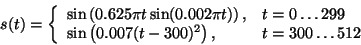$$s(t) = \left \{\begin{array}{ll} \sin \left ( 0.625 \pi t \s... ...(t - 300)^2 \right ), &t=300\ldots 512\\ \end{array} \right .$$ (7)

The upper plot of figure 3 presents the result of decomposition of this signal over a large dictionary ( $7.5 \times 10^5$ Gabor functions). In spite of the high resolution of this decomposition, the changing frequency is represented by a series of structures since all the dictionary's functions have constant frequency. The middle plot of Figure 3 shows an average of 50 time-frequency representations constructed from decompositions over different realizations of small ( $1.5 \times 10^4$) stochastic dictionaries. Their size was optimized for this particular signal, and the number of averaged decompositions was chosen to make the computational costs of both representations equal (compare section II). The plot in the middle panel corresponds better to Equation 7. However, it is constructed from 50 times more waveforms than the upper plot, so the underlying parametrization is not compact.

Figure 3: Energy density ( $E f ( t, \omega )$, eq. (5), proportional to shades of gray) of a simulated signal (bottom plot), calculated from single MP decomposition over a dictionary containing $7.5 \times 10^5$ waveforms (top) and averaged over 50 decompositions in different realizations of stochastic dictionaries, containing $1.5 \times 10^4$ atoms each (middle plot).